In the last level, we saw how U-SQL deals with indexing and partitioning. We covered off all of the key aspects of vertical partitioning, but only dealt with part of the horizontal partitioning picture. This article is going to fill in the gaps.

I’m going to run all of these queries locally, but feel free to run them directly against Azure if you wish.

A Quick Partitioning Recap

Vertical partitioning in Azure Data Lakes allows you, the developer, to control the partitions. You can add and drop partitions to or from a table. You specify the partition keys and U-SQL returns data from the appropriate partitions when requested. Horizontal partitions sees Azure Data Lakes take control of partitioning, with you providing the keys that tell the Data Lake how to partition data. There are four types of distribution schemes used by horizontal partitioning:

• HASH (keys) - We covered HASH in some detail in the previous article. You provide a column (or columns) to be used as the hash key in the U-SQL statement, and Azure Data Lakes deals with the partitioning of your data. If you want to see this in action, go and check out Level 6.
• DIRECT HASH (ID) - This is for developers who want to have some control over how the data is hashed. You need to specify an additional ID column in your table, and populate it using one of U-SQL’s windowing functions. We’ll see how this works in a little while.
• RANGE (keys) - If you are constantly using data ranges in your U-SQL queries, this distribution scheme could be a good option. It works to keep ranges of values together, making data retrieval faster as you specify ranges. We’ll use latitude and longitude to show this one off.
• ROUND ROBIN - The simplest of all distribution schemes. With this, you don’t specify any columns, you don’t pass go, and you definitely do not collect $200 (apologies if you’ve never played Monopoly and have no idea what I’m talking about!). Instead, the Azure Data Lake simply spreads your data evenly across the extents created for your file. This is an ideal solution when there is no obvious way to partition your data and U-SQL/Azure is telling you that you are having data skew problems. We’ll look at this one last of all.

We'll now give a bit more info on each of these types of partitions.

DIRECT HASH (ID)

OK, time to look at a distribution scheme. Kick up Visual Studio and open the SSC_UkPostcodes project we’ve been using (head on back to article 4 if you need to refresh yourself on this). Add a new script called 140 Create Postcodes_DirectHash Table.usql and add this code, which will create a new table.

USE DATABASE UkPostcodes;
USE SCHEMA Postcodes;
CREATE TABLE IF NOT EXISTS Postcodes_DirectHash
(
 Postcode string,
 CountyCode string,
 DistrictCode string,
 CountryCode string,
 Latitude decimal?,
 Longitude decimal?,
 DirectHashValue long,
 INDEX idx_Postcodes 
 CLUSTERED(Postcode)
 DISTRIBUTED BY DIRECT HASH (DirectHashValue) INTO 5);

This looks almost exactly the same as the Postcodes table we’ve created in previous articles, except for the last four lines.

DirectHashValue long,
INDEX idx_Postcodes
CLUSTERED(Postcode)
DISTRIBUTED BY DIRECT HASH (DirectHashValue) INTO 5

The first line here adds a column we haven’t seen before – it’s a completely custom column called DirectHashValue, which will store a numeric value. Lines two and three should look familiar, as should line four – except we’ve specified a DIRECT HASH is to be used for partitioning. The DIRECT HASH will work on the new column we’ve just added, and will be split across five extents.

Run this to create the table. Nothing magical or new happens, we just have a new table called Postcodes_DirectHash. Now we can populate this table.

Add another new U-SQL script, calling this one 150 Insert Postcodes_DirectHash Data.usql. The INSERT script we’re going to use should look familiar to you, with two exceptions – we’re using our first ever windowing function, and we’ve nested the EXTRACT statement, instead of assigning it to a rowset variable as we’ve done in previous articles.

USE DATABASE UkPostcodes;
USE SCHEMA Postcodes;
DECLARE @DataFilePath string = "/ssc_uk_postcodes/postcodes/Postcodes.csv";
INSERT INTO Postcodes_DirectHash
(
Postcode,
CountyCode,
DistrictCode, 
CountryCode, 
Latitude, 
Longitude, 
DirectHashValue 
)
SELECT
  Postcode, 
  CountyCode, 
  DistrictCode, 
  CountryCode, 
  Latitude, 
  Longitude, 
  Convert.ToInt64(DENSE_RANK() OVER (ORDER BY CountyCode)) AS DirectHashValue 
FROM (
      EXTRACT 
        Postcode string, 
        CountyCode string, 
        DistrictCode string, 
        CountryCode string, 
        Latitude decimal?, 
        Longitude decimal?
      FROM @DataFilePath USING Extractors.Csv()) AS PcodeData;

The nested EXTRACT can be clearly seen – we have a FROM (EXTRACT) statement. We’re essentially using the EXTRACT as a table. This works similarly to nested SELECT statements in T-SQL. What about the windowing function? Let’s take a look at this line in more detail:

Convert.ToInt64(DENSE_RANK() OVER (ORDER BY CountyCode)) AS DirectHashValue

Convert.ToInt64 is a C# casting method, which will ensure the value generated within the brackets will be returned as an INT64, also known as a long (to me, it’s just a very, very big number). Inside the brackets is a new U-SQL term we haven’t seen before – DENSE_RANK(). This works in the same way the T-SQL version does, giving rows a rank depending upon CountyCode ordering. All of the windowing functions you know and love from T-SQL are available in U-SQL. Here’s a few to whet your appetite, which we’ll investigate in a later article:

• COUNT
• SUM
• RANK
• DENSE_RANK
• NTILE
• ROW_NUMBER

Run this to populate the table. Now we’re in a position to see exactly what the DIRECT HASH(ID) partition scheme gives us. Add another new script and call it 160 Extract Postcodes_DirectHash Data.usql. Add this code to the new script.

USE DATABASE UkPostcodes;
USE SCHEMA Postcodes;
@allPostcodes = SELECT Postcode, CountyCode, DistrictCode, CountryCode, Latitude, Longitude, DirectHashValue
                FROM Postcodes_DirectHash;
                OUTPUT @allPostcodes TO "/outputs/dhPostcodes.tsv" 
                ORDER BY Longitude ASC USING Outputters.Tsv();

An extremely simple output query – we’re just going to grab everything from the Postcodes_DirectHash table. Hit the Submit button to fire this query in Visual Studio.

Once this has executed, and assuming you’ve executed this locally, the Local Run Results window should appear at the bottom of your screen, showing you the path to which the file has been saved. If you’ve ran this against Azure, you can navigate to the path using the Server Explorer or the Azure Portal.

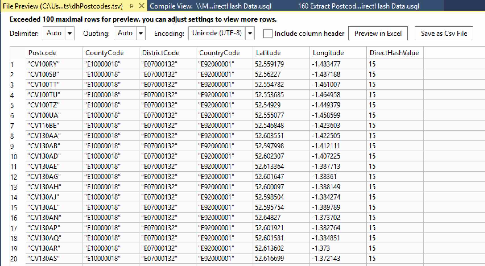
Right-click on the file name shown. Two options will be available – Preview and Open Location. Clicking on Preview gives you a handy display of the first 100 rows, along with a few options to change the delimiter and the quote settings. You can even save the modified file out as a CSV file or open it in Excel.

Take a look at the last column – DirectHashValue. It’s been populated with a number. To see just what numbers, we need to look at the entire file. Right-click on the file name in Local Run Results again, and click Open Location. This takes you to where your file was created, which in this case was in a sub-folder of the USQLDataRoot folder on your machine. This is automatically created for you and contains your local catalogs (databases) and output files.

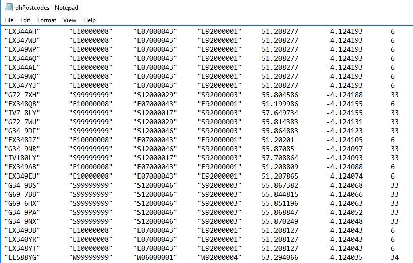
We’ll look at this in some detail in a future article. For now, let’s go back to the file we just created –  double-click the highlighted TSV file. It’s a bit big (70MB+), but after a moment it should open in Notepad or your favourite text editor. Scroll down until you see the value in the last column change – in the image below you can see 6, 33 and 34.

CountyCode is shown in column 2, with DistrictCode shown in column 3. If you remember, we ran the DENSE_RANK function over CountyCode. S99999999 is Scotland, which has been assigned a rank of 33; 34 is Wales (W99999999); and 6 is Devon (E10000008). Each individual CountyCode has been assigned its own rank.

The really useful thing here is you could assign a rank across multiple columns to define a really fine grain (CountyCode and DistrictCode, to name one example). How fine you want to go is up to you, but this is a powerful feature that gives you a lot of control over the way your data is partitioned.

RANGE (KEYS)

This scheme ensures ranges of values are kept together. You can partition on multiple columns if you wish. You provide the columns you want to partition on and U-SQL will figure out how best to partition your data based on those columns. This works in a similar fashion to the hashing mechanism we looked at in our previous article, except this time U-SQL and Azure Data Lakes are doing the heavy lifting, and we’re trusting them to do so.

We’ll create a range on Latitude and Longitude. Add another new script to the Visual Studio project, 170 Create Postcodes_Range Table.usql. Here’s the code to create that table:

USE DATABASE UkPostcodes;
USE SCHEMA Postcodes;
CREATE TABLE IF NOT EXISTS Postcodes_Range 
(Postcode string, 
CountyCode string, 
DistrictCode string, 
CountryCode string, 
Latitude decimal?, 
Longitude decimal?, 
INDEX idx_Postcodes CLUSTERED(Postcode) 
DISTRIBUTED BY RANGE(Latitude, Longitude));

This table looks just like the other Postcodes tables we’ve created, except (except!) for the penultimate line, which creates our range. It’s pretty simple to specify:

DISTRIBUTED BY RANGE(Latitude, Longitude)

Nothing to explain here really, just specify the RANGE keyword and the columns you want to partition on. Run this to create the table and then add another new script, to insert some data into the table. This will be called 180 Insert Postcodes_Range Data.usql. The code is exactly the same as script 150, except we’re inserting into the Postcodes_Range table and there isn’t a DirectHashValue column.

USE DATABASE UkPostcodes;
USE SCHEMA Postcodes;
DECLARE @DataFilePath string = "/ssc_uk_postcodes/postcodes/Postcodes.csv";
INSERT INTO Postcodes_Range 
(Postcode, 
CountyCode, 
DistrictCode, 
CountryCode, 
Latitude, 
Longitude) 
SELECT Postcode, CountyCode, DistrictCode, 
       CountryCode, Latitude, Longitude 
FROM (EXTRACT Postcode string, CountyCode string, DistrictCode string, 
      CountryCode string, Latitude decimal?, Longitude decimal? 
      FROM @DataFilePath USING Extractors.Csv()) AS PcodeData;

Run this to populate the table. Finally, we’ll create a script to return some data. Add one more script, calling it 190 Extract Postcodes_Range Data.usql. Yonder lies the code:

USE DATABASE UkPostcodes;
USE SCHEMA Postcodes;
@rangePostcodes =
  SELECT Postcode,
    CountyCode,
    DistrictCode,
    CountryCode,
    Latitude,
    Longitude
  FROM Postcodes_Range
    WHERE CountyCode == "E10000017"
      AND Latitude BETWEEN (decimal)53.55 AND (decimal)53.56
      AND Longitude BETWEEN (decimal)-2.905 AND (decimal)-2.900;
  OUTPUT @rangePostcodes
    TO "/outputs/rangePostcodes.tsv"
  USING Outputters.Tsv();

There are some interesting things going on in this script, specifically in the WHERE clause. We’re firstly filtering on the CountyCode for Lancashire, before requesting some particular Latitude and Longitude ranges. We can write any type of query we like, but as we’re using the RANGE operator I thought I’d take this chance to demonstrate how we can request a range in U-SQL. I’m sure most of you will already know and love the BETWEEN keyword, but you might be surprised to see the (decimal) in front of the numbers. This is a C# cast, and it is explicitly telling U-SQL to treat these numbers as decimals. If this cast is not present we’d see this error:

This tells us U-SQL, just like T-SQL, is converting the BETWEEN keyword to >= and <=. The actual complaint is that the operator can’t be applied to columns with a data type of decimal?. We first met this in Level 5 – the question mark denotes this is a decimal column that also supports NULL values. In this case, it’s the nullability which prevents the compiler from using the column for the BETWEEN clause, hence the cast to a standard, non-nullable decimal. We’re safe to use this here as I know there are no NULL values in this columns – if there were you’d need to filter them out before running the query.

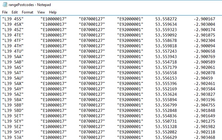
Run the script and a new file called rangePostcodes.tsv will be created, containing the results. You can right-click on the file name shown in the Local Run Results window that has appeared, just like we did earlier. Only 36 records matched our criteria.

With the RANGE distribution scheme, you’re handing some control over to U-SQL and the Azure Data Lake. You’re controlling which columns the data is split on, but Azure is controlling exactly how the data is partitioned. With some experimentation, this may turn out to be just the scheme you need.

ROUND ROBIN

This is the simplest partition scheme. You may have noticed that as we’ve looked at each scheme we’ve gradually handed more control over to U-SQL. With Round Robin, you hand over total control. This simply splits the data evenly across a number of partitions. This could slow down some queries and speed up others, depending upon how many extents/partitions have to be accessed to obtain all of the necessary data.

We won’t go into a detailed example with this one, but it’s very simple. When you create your table, you specify PARTITIONED BY ROUND ROBIN. The big difference is you don’t provide any columns or keys – there’s no need to. Here’s a CREATE TABLE statement to prove it:

  CREATE TABLE IF NOT EXISTS Postcodes_RoundRobin
  (
  Postcode string,
  CountyCode string,
  DistrictCode string,
  CountryCode string,
  Latitude decimal?,
  Longitude decimal?,
  INDEX idx_Postcodes
  CLUSTERED(Postcode)
  DISTRIBUTED BY ROUND ROBIN
  );

You can populate and query this table just like any of the other tables we’ve created. You may notice some speed differences with some of the queries, depending upon what you’re querying for.

Now, I suspect you may be thinking – why the heck would I ever use this? I’ll always know my partition columns. Well, that might well be true. But what if your chosen partition scheme leads to something called Data Skew? What would you do then? This is the problem ROUND ROBIN tries to solve.

Data Skew

In the last article, we discussed what a vertex is. It represents a unit of work in U-SQL. We learnt that vertices can time out after five hours. This timeout is involved in data skew. Let’s look at an example.

• Assume we’ve partitioned using the CountyCode column
• Assume we have a record for every person in the UK – roughly 64 million records
• A large number of those records are centred around a few key areas – London has 8.6 million residents, and Manchester has 2.5 million, for example
• Some areas don’t have many residents at all (relatively) – Cumbria has 500,000, for instance

If we run a query on this data, we have an imbalance. The data retrieved from the Cumbria partition may be returned relatively quickly, but we’ll have a long wait for the London data, which is over 17 times larger. This is data skew, where a single vertex handles all rows that match a particular key. There’s another scenario that can lead to excessively large vertices – limited distinctiveness. If you’re filtering on a key with a small number of values (e.g. Cat, Dog), this could also lead to vertices timing out.

To resolve these issues, you need to either change your partitioning approach, or choose keys that have a larger number of distinct values. In the CountyCode case up above, we could change the scheme to use DistrictCode as well. This would spread the data wider, reducing the time it would take vertices to complete.

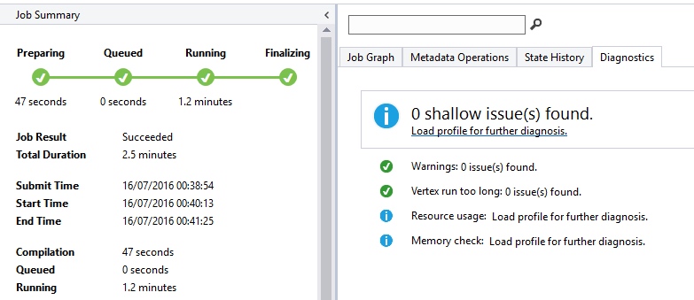
Fortunately, you don’t have to figure all of this out by yourself. Should you run into data skew or other similar problems, Visual Studio can tell you all about it. You need to run the query directly against Azure for this to work. Run the job, and once it completes click on the Diagnostics tab in the Job View window that appears.

Visual Studio tells you if Azure found any shallow issues you may need to deal with. These include data skew issues, memory issues and resource issues. From the information given, you’ll be able to investigate further and resolve the issue. Helpful, isn’t it?

Summary

This article concludes our tour of the various partitioning and distribution schemes provided by the Azure Data Lake and U-SQL. We’ve covered all of the key aspects. We’ve seen across most of the articles so far how we can query data from a single file or table. However, as SQL practitioners, we know much of the power of SQL comes from its ability to return data from multiple data sources, using JOINs and other similar constructs. Well, you’ll be delighted to know JOINs are alive and kicking in U-SQL, and we’ll take a good look at these next time out. See you then!