We’ve covered almost all of the key database objects available to you in U-SQL. Tables, views, schemas, table-valued functions (TVFs) and the like. We’re now going to complete the set of core objects by taking a look at the venerable stored procedure. You’ll notice these are pretty similar to T-SQL stored procedures, but with the usual U-SQL quirks. Along the way, we’ll see how U-SQL supports the TOP n clause, NULL equality and simple aggregation using SUM.

What Can You Do with a Stored Procedure?

On the surface, stored procedures are similar to TVFs. Both types of object support parameters, can contain more than one statement, and can reference user code. The big difference comes in what they can (or cannot) return. A TVF can return results, but a stored procedure cannot. A TVF can return a table, but a stored procedure can only output to a file or modify the data in a table.

Stored procedures are great for encapsulating code, such as a loading process. You can even have the procedure output to multiple targets if you wish, e.g. to a file and a table. Which, funnily enough, is what we’re going to do in this very article.

The Example Stored Procedure

The example stored procedure we’re going to create in this article will return an aggregated result set, showing how many males, females and occupied households there are for each individual county and district combination. It will do this using the following implementation:

• Accept two parameters – one which allows the caller to specify how many rows to return, and another to filter the results to an individual county
• Check if a table exists to store the output. If it does, drop it. Then recreate the empty table
• Obtain the base data set
• Generate the aggregated data set
• Output the results to a file
• Insert the results into the table we created

Before we can create the stored procedure, let’s ensure the tables are populated with data.

Obtaining the Data Files

To obtain the latest version of the data files, along with the code, go to the Stairway’s GitHub project and download the code. You’ll find the data files in the ssc_uk_postcodes folder.

Populating the Tables

In the GitHub project, open up script 200 Populate Tables.usql. If you have already created the tables, running this will repopulate them (I’ve added the TRUNCATE TABLE statement here, which U-SQL supports). If you haven’t created the tables (or, indeed, the database), run scripts 010 to 060 first. All done? Cool, let’s create a stored procedure!

Creating and Dropping a Stored Procedure

If you’ve pulled the code from GitHub, open the solution in Visual Studio 2015. You’ll already have script 500 Create GenerateAreaStatistics Procedure.usql. If you don’t have it and you’ve been following along, open your own solution and create an empty script with the same name.

I’m sure the first few lines of the script won’t shock you:

USE DATABASE UkPostcodes;
USE SCHEMA Postcodes;
DROP PROCEDURE IF EXISTS GenerateAreaStatistics;
CREATE PROCEDURE IF NOT EXISTS GenerateAreaStatistics
(@NoRowsRequired int = 0, @TargetCounty string = null)
AS
BEGIN;

Yes, our old friends DROP and CREATE are back. They work just like all the other CREATE and DROP statements we’ve discussed in previous articles, so I won’t go into detail about them here.

The Area Statistics Stored Procedure

If you’ve just created a blank script 500, paste this code into it. This is the entire code for the stored procedure – we’ll work through what it does in a moment.

USE DATABASE UkPostcodes;
USE SCHEMA Postcodes;
DROP PROCEDURE IF EXISTS GenerateAreaStatistics;
CREATE PROCEDURE IF NOT EXISTS GenerateAreaStatistics
(@NoRowsRequired int = 0, @TargetCounty string = null)
AS
BEGIN;
DECLARE @NoRowsToReturn int = @NoRowsRequired <= 0 ? 1000000 : @NoRowsRequired;
DROP TABLE IF EXISTS AreaStatistics;
CREATE TABLE IF NOT EXISTS AreaStatistics
(
CountyName string,
DistrictName string,
NoMales Int64?,
NoFemales Int64?,
NoOccupiedHouseholds Int64?,
INDEX idx_TableStats
CLUSTERED(CountyName, DistrictName) DISTRIBUTED BY HASH(CountyName)
);
@basedata =
SELECT c.CountyName, d.DistrictName, pe.Males, pe.Females, pe.OccupiedHouseholds
FROM Postcodes AS p
INNER JOIN Counties AS c ON p.CountyCode == c.CountyCode
INNER JOIN Districts AS d ON p.DistrictCode == d.DistrictCode
INNER JOIN PostcodeEstimates AS pe ON p.Postcode == pe.Postcode;
@calculateddata =
SELECT CountyName, DistrictName, SUM(Males) AS NoMales, SUM(Females) AS NoFemales,
SUM(OccupiedHouseholds) AS NoOccupiedHouseholds, SUM(Males) + SUM(Females) AS TotalNoPeople
FROM @basedata
WHERE (CountyName == @TargetCounty OR @TargetCounty IS NULL)
GROUP BY CountyName, DistrictName
ORDER BY CountyName, DistrictName
FETCH FIRST @NoRowsToReturn ROWS;
OUTPUT @calculateddata
TO "/outputs/statistics.csv"
ORDER BY CountyName ASC, DistrictName ASC
USING Outputters.Csv();
// Insert data into table
INSERT INTO AreaStatistics
(CountyName, DistrictName, NoMales, NoFemales, NoOccupiedHouseholds)
SELECT CountyName, DistrictName, NoMales, NoFemales, TotalNoPeople
FROM @calculateddata;
END;

The code isn’t that big, but it does a lot. Let’s take a look at each piece of the puzzle.

Parameters

Just like TVFs, stored procedures can accept parameters – both mandatory and optional. This stored procedure declares itself with two optional parameters:

CREATE PROCEDURE IF NOT EXISTS GenerateAreaStatistics
(@NoRowsRequired int = 0, @TargetCounty string = null)

@NoRowsRequired will, if specified, limit the number of rows processed by the stored procedure (we’ll be introduced to U-SQL’s version of TOP very shortly). @TargetCounty offers a filter – if it’s passed, only values for the specified county will be processed, otherwise all counties will be processed. When we created the optional parameter in the TVF (in the previous article), we specified a string constant – this time we’ve used NULL. NULL is what you’ll normally use, and it works in a similar fashion to T-SQL nulls.

U-SQL only supports input parameters – you won’t find any output parameters here.

Modifying Parameter Values

The first line of “real” code in the SP declares a variable.

DECLARE @NoRowsToReturn int = @NoRowsRequired <= 0 ? 1000000 : @NoRowsRequired;

This sets the value of a new variable, @NoRowsToReturn. It checks the @NoRowsRequired input parameter value. If this is equal to or less than zero, it defaults to 1,000,000 – otherwise it uses the value passed in, e.g. 10. It uses the conditional/ternary operator we first met in article 9. But why, when we already have a parameter, did we have to declare a new variable to store this? Why couldn’t we just write something like:

SELECT @NoRowsRequired = @NoRowsRequired == 0 ? 1000000 : @NoRowsRequired;

We couldn’t write the code like this, because U-SQL complains very loudly:

The key error is the last one - @NoRowsRequired is not assignable. Yep, I’m afraid input parameters are read-only.

Executing DDL Inside a Stored Procedure

Now, if you were writing this for real, it’s highly likely you’d have created a table to store the statistic results using a separate script. But I’m trying to show off what U-SQL can do, so I’ve popped all of the table processing in here! Yes folks, the next piece of code drops the table if it exists, then recreates it.

DROP TABLE IF EXISTS AreaStatistics;
CREATE TABLE IF NOT EXISTS AreaStatistics
(
CountyName string,
DistrictName string,
NoMales Int64?,
NoFemales Int64?,
NoOccupiedHouseholds Int64?,
INDEX idx_TableStats
CLUSTERED(CountyName, DistrictName) DISTRIBUTED BY HASH(CountyName)
);

This is stuff we’ve seen before (and if you haven’t seen it, run back to article 5 – we’ll wait for you). It’s just a bit unique because we’re doing it in a stored procedure.

Obtaining the Base Data Set

This next statement will also look familiar to long-time U-SQL Stairway readers. We’re grabbing a row set, which we can use as the basis for our statistics.

@basedata =
SELECT c.CountyName, d.DistrictName, pe.Males, pe.Females, 
pe.OccupiedHouseholds 
FROM Postcodes AS p
INNER JOIN Counties AS c ON p.CountyCode == c.CountyCode
INNER JOIN Districts AS d ON p.DistrictCode == d.DistrictCode
INNER JOIN PostcodeEstimates AS pe ON p.Postcode == pe.Postcode;

Coo-el. Well, not really – it’s a pretty boring query which returns the columns we’re interested in. Even the joins fail to raise any excitement. But hey, we have the core data we need, which means our next statement is super exciting!

Aggregating and Limiting the Data

We performed a simple COUNT in article 3 of this series, but now we’ll see some real aggregation for the first time. On top of that, we’ll also see how U-SQL limits its results sets too! Hold on to your hats:

@calculateddata =  
SELECT CountyName, DistrictName, SUM(Males) AS NoMales, 
SUM(Females) AS NoFemales, SUM(OccupiedHouseholds) AS NoOccupiedHouseholds, 
SUM(Males) + SUM(Females) AS TotalNoPeople
FROM @basedata
WHERE (CountyName == @TargetCounty OR @TargetCounty == null)
GROUP BY CountyName, DistrictName
ORDER BY CountyName, DistrictName
FETCH FIRST @NoRowsRequired ROWS;

We’re pulling the data from @basedata and assigning the aggregated set to @calculateddata. Look at the SUM statements – they’re just the same as T-SQL. You can COUNT and perform other aggregations too – we’ll look at all of the options in a future article. GROUP BY does the same job as its T-SQL brother.

NULL Equality

The WHERE clause in the above statement filters the results if a county name has been passed in. If no county name has been passed in, it returns everything by checking if the variable value is NULL:

@TargetCounty == null

We don’t use IS NULL as we do in T-SQL, but rather == null. However, you may be amazed to learn that you could also have written it as:

@TargetCounty IS NULL

Both statements are functionally equivalent, so feel free to use which is best for you. Likewise, to check if something is not null, you can write:

@TargetCounty != null

Or:

@TargetCounty IS NOT NULL

Limiting the Number of Rows

The last line of the aggregation statement shows how U-SQL implements the TOP clause we all know and love from T-SQL. U-SQL uses FETCH FIRST rather than TOP:

FETCH FIRST @NoRowsToReturn ROWS;

The beauty of this is we can pass in a parameter to specify how many rows to return (just like the TOP clause in SQL Server since 2005). Unlike T-SQL, the limiter goes at the end of the statement, not the start. This will return the first N rows, as dictated by the ORDER BY statement. We could also have written:

FETCH LAST @NoRowsToReturn ROWS;

Which, as I’m sure you’ll have gathered, would return the last N rows, effectively reversing the ORDER BY. These are powerful options, giving U-SQL an elegant flexibility.

Writing Data to a File

At this point, we have all the data we need, in the format we want it in. It’s been aggregated and limited. So we use what should (by now) be the familiar OUTPUT statement to write the data to a file. I’ve shown the ORDER BY here as a reminder that ordering can be performed when writing to a file, but this statement doesn’t need it – the SELECT statement that assigned rows to @calculateddata already applied the sort.

OUTPUT @calculateddata
TO "/outputs/statistics.csv"
ORDER BY CountyName ASC, DistrictName ASC
USING Outputters.Csv();

This leaves us with one final statement – to insert the data to a second target – a database table.

Executing DML Inside a Stored Procedure

We saw how to create a table using DDL inside the stored procedure earlier – let’s have a look at using DML to insert data into that table. Again, this is a command we’ve met earlier in the Stairway.

// Insert data into table
INSERT INTO AreaStatistics
(CountyName, DistrictName, NoMales, NoFemales, NoOccupiedHouseholds)
SELECT CountyName, DistrictName, NoMales, NoFemales, TotalNoPeople
FROM @calculateddata;

That’s just about it! All we need is a closing END statement and we’re done.

Creating the Stored Procedure

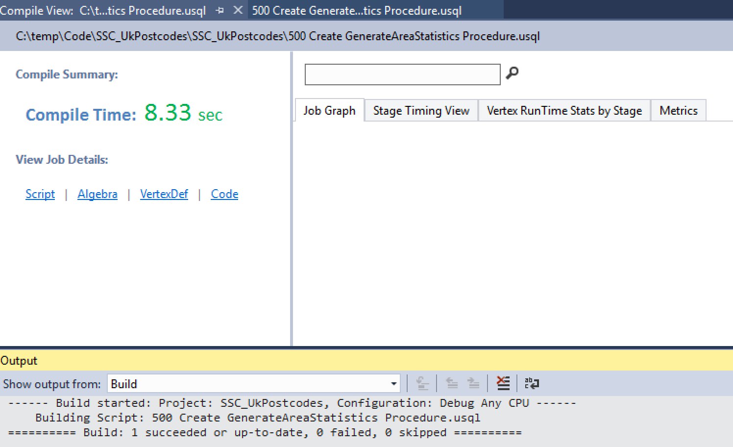
To create your stored procedure, make sure script 500 is open. Then just hit the Submit button on the U-SQL toolbar.

Using the Stored Procedure

Creating a stored procedure is all well and good, but it isn’t much use to us just sitting in a database. Happily, it’s as easy to use a stored procedure in U-SQL as it is in T-SQL. If you downloaded the code from GitHub, you already have script 510 Execute AreaStatistics.usql. If you don’t have it, create it. Here’s the code:

USE DATABASE UkPostcodes;
USE SCHEMA Postcodes;
GenerateAreaStatistics
(200, DEFAULT);

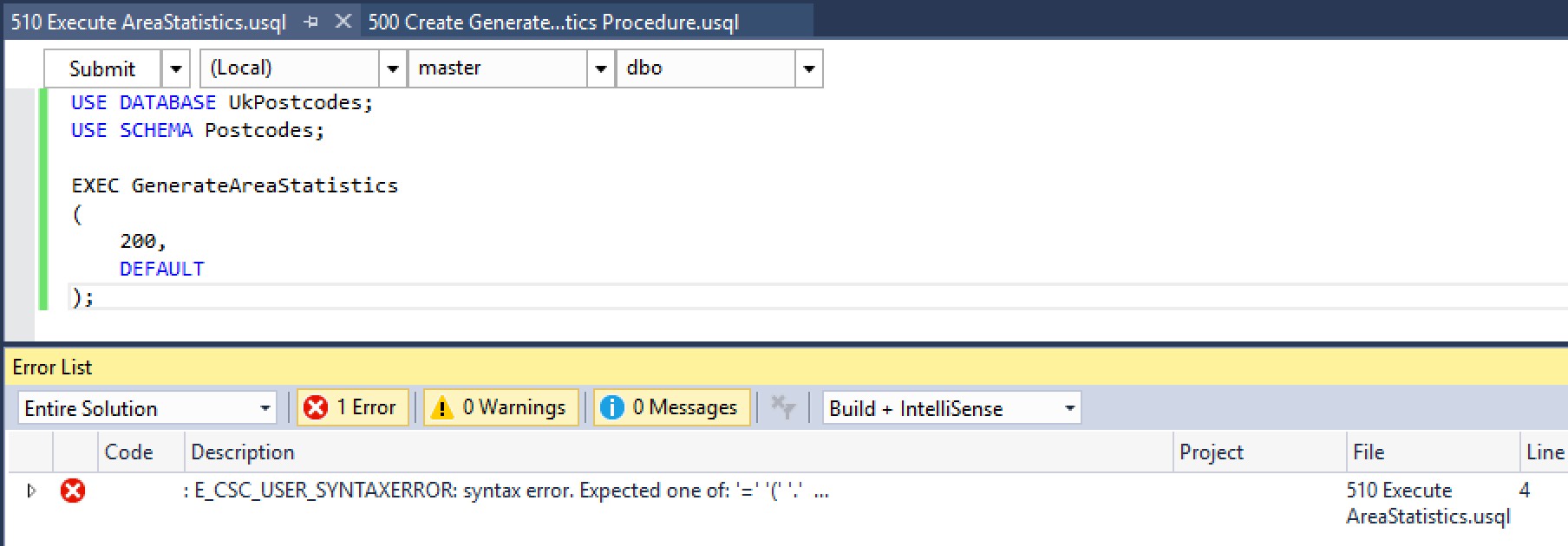
We don’t need an EXEC statement (U-SQL doesn’t have an EXEC statement). If you try to use EXEC you’ll notice two things – the EXEC keyword isn’t picked up as an Intellisense keyword, and your script fails.

If we run it without EXEC, everything is tickety-boo. Note the parameters (in the image above) – we’ve asked the procedure to return up to 200 rows, for all areas (DEFAULT).

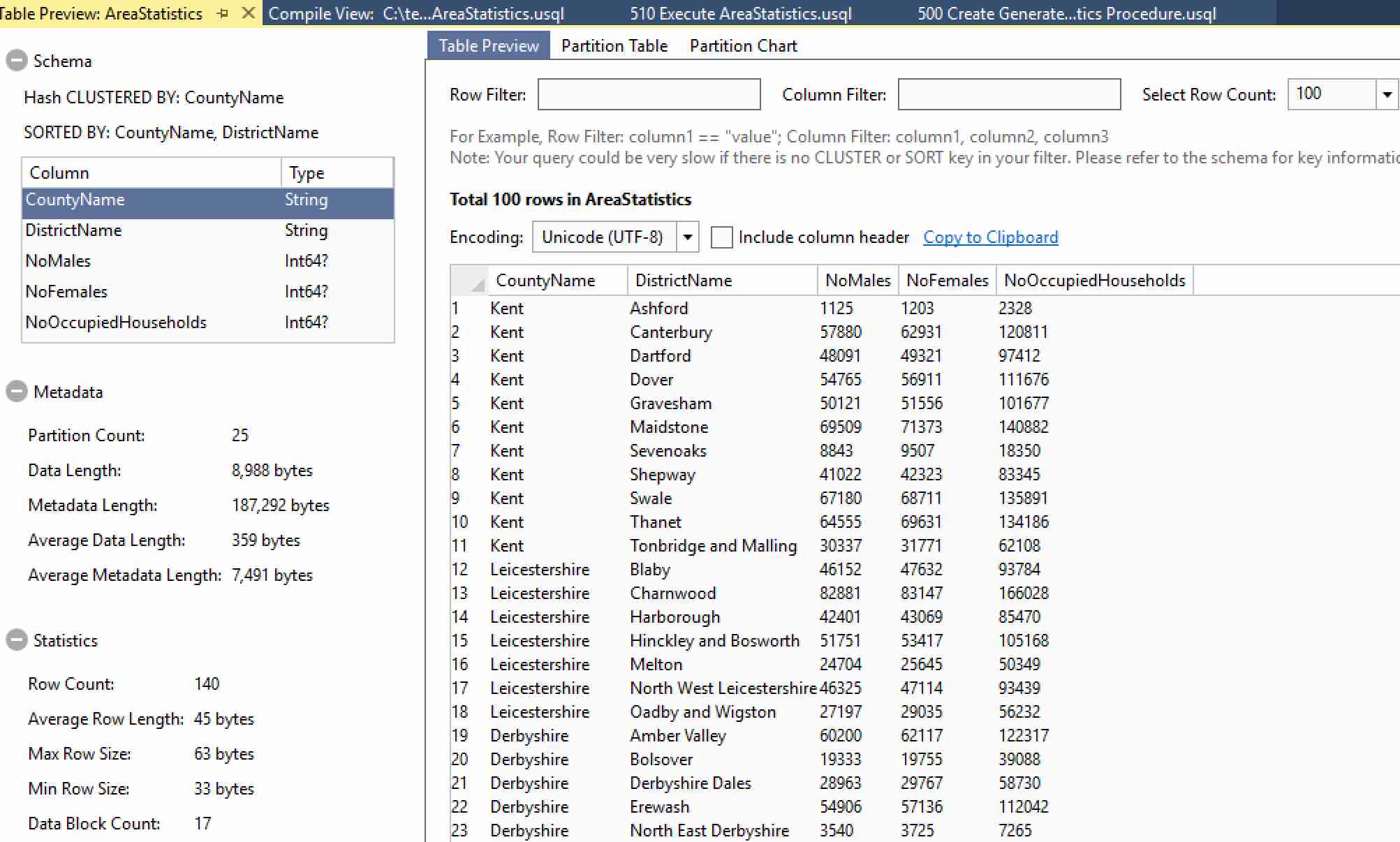
So, what do we see once the procedure has executed? Not only do we have a nice graph in the output, we also have TWO (count ‘em, TWO) local run results! The first one is our table, the second is our file. Right-click on the first row (the table). There are two options – Preview and Open Location. Open Location does nothing – this is a table, so there is no file location. With that in mind, click on Preview and you’ll be treated to a pleasant view of your table.

There’s a whole raft of data available here. You can find out how many partitions your table has, how many rows are in the table and what the minimum/maximum row sizes are, amongst other things. Try clicking on the Partition Table and Partition Chart tabs along the top – there’s plenty more partition goodness available to you there too!

The Stored Procedure File Output

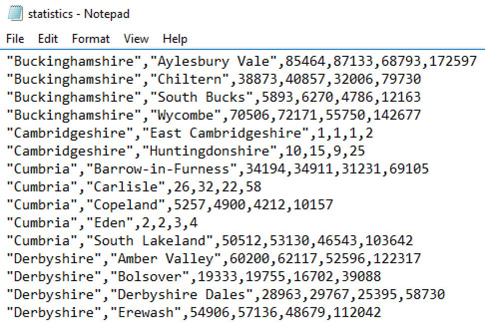
Finished analysing the table? Good! To finish off, click on Local Run Results again. This time, right-click on the second row (the statistics.csv file) and choose Open Location. This will open Windows Explorer, with the CSV file highlighted. Double-click on it to open it in Notepad, Excel or whatever editor you use.

So, with one relatively simple stored procedure we’ve generated some useful statistics and written them to two outputs. Very powerful, very reusable, and very impressive.

Summary

That’s about it for this time. We’ve seen how stored procedures are implemented in U-SQL, and we’ve walked through an example stored procedure which shows how quickly something fairly complicated can be put together.

We’ve now covered all of the core database objects in U-SQL. There are some other objects, such as Data Sources, that we’ll investigate in the fullness of time. But we have seen all of the stuff you are likely to use on a day-to-day basis.

We’ll change tack in the next article, and meet two new data types provided by U-SQL – SQL.MAP and SQL.ARRAY. It’s interesting stuff, so be sure to come back! See you then.