In this Level, we will conclude the series of steps surrounding the general MDX member functions I began in Level 5: Members, and an Introduction to the MDX Members Functions. In particular, we’ll concentrate upon the .LastSibling and Cousin() functions. For each of these, we’ll discuss the syntax with which we employ it, its operation in general and the datasets it returns. We’ll then get some hands-on exposure to each function, first creating queries that let us see it in action, and then analyzing data sets that the queries return, to reinforce a practical understanding of the function.

Let’s take a look at each of these two “family” functions individually, as we have with others in previous Levels, beginning with .LastSibling function.

The .LastSibling Function

The .LastSibling function resembles the .FirstSibling function in its capacity to induce confusion to those new to MDX: the way that it behaves with the last child of a given member-parent is the interesting part: like .FirstSibling, the .LastSibling function operates within a “horizontal” scope from the perspective of the hierarchy to which it belongs. Its behavior mimics “travel” within the same level of the hierarchy (“across,” again unlike the .FirstChild and .LastChild functions that we explored in earlier steps).

The relationships under consideration might be better understood with a little visual assistance. As in earlier steps, we’ll consider the Date dimension for this illustration because we all understand the hierarchy (without necessarily understanding the structure of the sample Adventure Works organization), and can therefore focus on the core concept instead of the structure of the hierarchy we rely upon as an example.

We will rely heavily upon the Date dimension in illustrating the syntax and use of the “family” functions for another reason we have cited in other examples: the Date dimension, composed of years, semesters, quarters, months, and so forth, works well with Cousin(), because, in most cases, an identical number of descendant members reside under any given ancestor. This scenario provides an excellent basis for using MDX “family” functions. There are certainly exceptions, but, for the most part, the Date dimension is about as predictable as it gets, with regard to consistency in arrangement.

An illustration of the use of the .LastSibling structure to which I refer appears here:

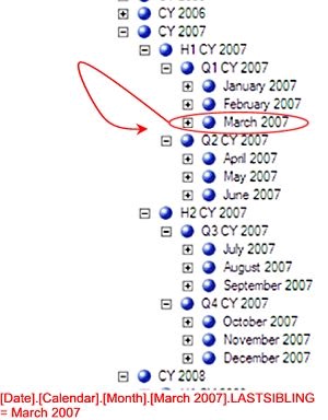
Illustration 01: .LastSibling in the Now-Familiar Date.Calendar Dimension Hierarchy

Once again, we are confronted with a possibly confusing scenario: the last child (March 2007 in the example illustrated above) also fills the role of last sibling – it is “last” within the horizontal level, and is the last sibling of any member residing at the same level, as well.

To amplify the concept with another illustration, let’s examine the relationships when we consider the last sibling of February 2007.

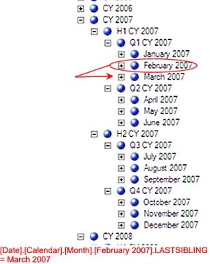
Illustration 02: Last Sibling for February 2007 is March 2007 …

We see in the illustration above that the last sibling of February 2007 is March 2007 – the last member in the level. .LastSibling works exactly like .FirstSibling, just in a “different direction” horizontally.

Syntactically, the .LastSibling function is appended to the right of the member, as shown in the following:

<member>.LastSibling
A simple example of the .LastSibling function in action follows:
SELECT
{[Date].[Calendar].[Calendar Year].[CY 2007].LASTSIBLING}
ON COLUMNS
FROM
[Adventure Works]
WHERE
([Measures].[Internet Sales Amount])

The dataset returned would appear as depicted:

Illustration 03: Example Result Dataset from Using the .LastSibling Function

The presence of the “empty” Calendar Year 2010, which resides “in the future,” from the perspective of the Adventure Works sample Analysis Services database, can be verified as the “last sibling” among the years. We can see it within the Date dimension structure on the Metadata tab of the Management Studio:

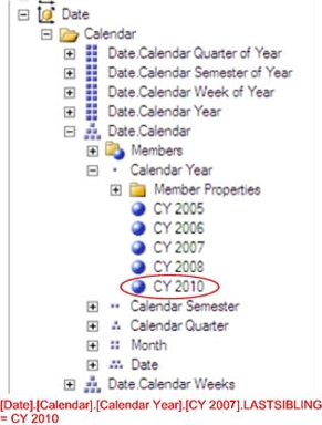
Illustration 04: CY 2010 is the “Last Sibling” in the Date Dimension Structure …

Let’s reinforce our understanding of how .LastSibling behaves by working another straightforward exercise. We’ll assume that a group of hypothetical client colleagues have presented us with a request: they’d like to see the total Internet Sales Amount for each of the Bike product categories for the last Quarter of Calendar Year 2007. They tell us that they ultimately intend to parameterize various components of the qualified name for members of the Date dimension, within reports that the query will support. They ask that we demonstrate a means, via an MDX function, options that are available, via MDX functions, to facilitate embedding the necessary report / query parameters.

We see this as an opportunity to demonstrate ways to use another MDX function, .LastSibling, and proceed to do so with the following steps. We will, as usual, work with the MDX Query Editor in SSMS. If you are not sure how to set up SSMS in Analysis Services to access the Adventure Works DW 2008R2 database, then click here for guidance.

Click / select the Adventure Works cube in the SSMS Object Explorer.

Click the New Query button above the Object Explorer.

Type (or copy and paste) the following query onto the new canvas of the Query pane that opens:

-- SMDX009-001: Basic Use of .LASTSIBLING
SELECT
{[Date].[Calendar].[Calendar Quarter].[Q3 CY 2007].LASTSIBLING}
ON AXIS(0),
{[Product].[Product Categories].[Category].[Bikes].CHILDREN}
ON AXIS(1)
FROM
[Adventure Works]
WHERE
([Measures].[Internet Sales Amount])

The query appears within the Query pane:

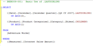
Illustration 05: Query Employing .LastSibling Appears in the Query Pane

Click the Execute (!) button in the toolbar, once again.

Analysis Services populates the Results pane:

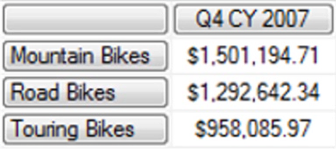
Illustration 06: The Query Results via the .LastSibling Function

The results dataset displays a summary of Internet Sales Amount for each constituent member of the Bikes product category for the fourth quarter of Calendar Year 2007, because we affixed the .Children function to the Bikes member of the category level, just as we did in the earlier exercise with .FirstSibling. As we have noted to be the case with other “family” functions in previous levels, we will find the .Children function far more powerful when used in combination with relative members, as Stairway to MDX evolves.

Save the query by selecting File Save MDXQuery1.mdx As …, naming the file SMDX009-001.mdx, and placing it, as we did with the queries we constructed earlier in this article, in a meaningful location.

Now, let’s try another query illustrating the co-operation of .LastSibling and the .Children function. This time, our colleagues have asked that we craft a query to return total Internet Order Quantity, associated with customer accounts in the United Kingdom, for the Touring bike product line, by month for the three months of the fourth quarter of Calendar Year 2007, using what we have learned thus far. Employing the .Children function again, we will enumerate the months contained within Q4 CY 2007, which we have determined in the query immediately above, to be the last sibling of member Q3 CY 2007 (the last of the peer members in its quarter horizontal level) of the Date dimension. To restate, our intent will be to create a column for each month in Q4 CY 2007 and a row for each child member of the Touring subcategory level of the Bikes product line.

• Select File New from the top menu, as we did earlier.

Select Query with Current Connection from the cascading menu that appears next, once again.

Type (or copy and paste) the following query into the Query pane:

-- SMDX009-002: .LASTSIBLING with .CHILDREN to Descend Another
-- "Generation"
SELECT
{[Date].[Calendar].[Calendar Quarter].[Q3 CY 2007].LASTSIBLING.CHILDREN}
ON AXIS(0),
{[Product].[Product Model Lines].[Product Line].[Touring].CHILDREN}
ON AXIS(1)
FROM
[Adventure Works]
WHERE
([Measures].[Internet Order Quantity],
[Customer].[Customer Geography].[Country].[United Kingdom])

The query appears in the Query pane:

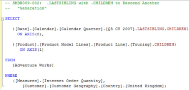
Illustration 07: The Query, with .LastSibling and .Children Combination

In addition to using the .Children function with another source member, once again, we are also expanding the WHERE statement: the idea is, of course, to specify not only the Internet Order Quantity measure, but a single customer Country, the United Kingdom. The cube is therefore filtered, or “sliced” for the Internet Order Quantity and the United Kingdom members (united, of course, in a tuple expression), within the context in which they are specified.

Click the Execute (!) button in the toolbar atop the Management Studio, once again.

Analysis Services returns the requested dataset:

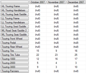
Illustration 08: The Query Results Dataset, Using the .LastSibling / .Children Combination

The results dataset displays the Internet Order Quantity totals for the children of the Touring bike product line, for the three months comprising Quarter 4 of Calendar Year 2007, as purchased by customers in the United Kingdom.

Save the query by selecting File Save MDXQuery2.mdx As …, naming the file SMDX009-002.mdx.

It comes as no surprise that the above results present an opportunity to make our presentation a bit more user-friendly to its ultimate audience: blank / null spaces often confuse information consumers (assuming, of course, that the consumers do not explicitly want to see the nulls). As we are well aware by this Level in our series, removing these spaces only requires a minor adjustment to the query.

Modify the comment lines (to reflect lines 1 and 2 of the syntax below), and add the keywords NON EMPTY to the far left of the rows specification (line 6) of the query we crafted above, as follows:

-- SMDX009-003: .LASTSIBLING with .CHILDREN to Descend Another
-- "Generation" [ADDING "NON EMPTY" TO ROW AXIS TO REMOVE EMPTIES]
SELECT
{[Date].[Calendar].[Calendar Quarter].[Q3 CY 2007].LASTSIBLING.CHILDREN}
ON AXIS(0),
NON EMPTY {[Product].[Product Model Lines].[Product Line].[Touring].CHILDREN}
ON AXIS(1)
FROM
[Adventure Works]
WHERE
([Measures].[Internet Order Quantity],
[Customer].[Customer Geography].[Country].[United Kingdom])

The modified query, with adjusted sections circled, appears within the Query pane:

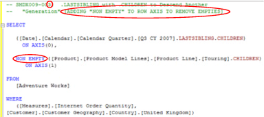
Illustration 09: The Query, with Our Modifications

Press F5 to execute the newly modified query.

The “leaner” dataset appears as depicted:

Illustration 10: Dataset Returned – “sans Empties …”

As with the query “pre-modifications,” the results dataset displays the Internet Order Quantity totals for the children of the Touring bike product line, for the three months comprising quarter 4 of Calendar Year 2007, as purchased by customers in the United Kingdom. But this time the empty intersects are removed, through the suppression action of the NON EMPTY keywords. As we have seen in earlier steps, Non Empty removes any tuples on the affected axis that are associated with empty intersects before the results are displayed.

Save the query by selecting File Save SMDX009-002.mdx As …, naming the file SMDX009-003.mdx.

Now that we’ve seen how to use the .FirstSibling and .LastSibling functions, let’s take a look at one more “family” member function, Cousin(), before concluding this Level .

The Cousin() Function

As we have shown in earlier sections of this Level, as well as in other Levels of this series (particularly in in Level 5: Members, and an Introduction to the MDX Members Functions), the capability to perform operations within the vertical and horizontal scopes of the hierarchy can mean more efficient, simpler MDX queries. The Cousin() function, like the .FirstSibling and .LastSibling functions we examined in earlier parts of this Level, belongs to the latter of the two general groups, as it returns a member that is “parallel” in position under a given ancestor member, as we shall see. We’ll take a look at the Cousin() function in this section, to obtain an appreciation for its capabilities.

Differences obviously exist between the functions. The most noticeable mechanical difference lies within the simple fact that the Cousin() function is applied differently than the .FirstSibling and .LastSibling functions, in that it is not “appended” to the source member. The source member (“Member_Expression”) is placed within the parentheses to the right of the word “Cousin,” as shown below:

Cousin( Member_Expression , Ancestor_Member_Expression )

The Cousin() function is written in standard MDX function format, which is to say Function(Arguments). The parentheses enclose the arguments, in this case the targeted member expression (designating the member for which we seek to return the cousin), and the ancestor member expression (representing the ancestor member upon whose “lineage” we wish to find the cousin member). The two members within the argument are separated by a comma.

Take a look at the syntax in the following example:

SELECT
{COUSIN([Date].[Calendar].[Month].[May 2007],
[Date].[Calendar].[Calendar Quarter].[Q4 CY 2007])}
ON COLUMNS
FROM
[Adventure Works]
WHERE
([Measures].[Internet Sales Amount])

The results dataset returned by this query would appear as shown:

Illustration 11: Example Result Dataset from Using the Cousin() Function

As we can see above, the Cousin() function within the example yields the member November 2007 (whose qualified name is [Date].[Calendar].[Month].[November 2007]). In the Adventure Works cube, as we might expect, the Q4 CY 2007 quarter level contains October 2007, November 2007, and December 2007. November 2007 is returned because it occupies the same relative position (the second child position) within the Calendar Quarter level as is occupied by May 2007 (again, the second child) in Q2 CY 2007.

A graphic view of the hierarchy for the source member ([Date].[Calendar].[Month].[May 2007]) within the function above will make the illustration more meaningful. In the illustration below, we see that May 2007 is a member of the Q2 CY 2007 sublevel of the CY 2007 Year level, within the Date dimension. The order of the members within the database determines the status of May 2007 as “second;” November 2007 is the second child member of the Q4 CY 2007 level. Therefore, when we specify in the second part of the function that we want the “same relative position for the Q4 CY 2007 level of the Date hierarchy,” the second child member (which happens to be November 2007, in this example) is returned.

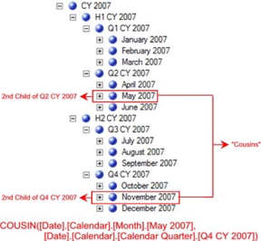
Illustration 12: Graphical Results of Using the Cousin() Function

In the simple example above, we can easily see that the cousin member is November 2007. As we shall observe, the Cousin() function returns the child member that occupies the same relative position, under its parent member, as the position under its own parent that the specified source member occupies. The operation of the function is based upon the order and position of members within levels.

Let’s construct an expression that calls the Cousin() function into action, to activate our understanding of how it operates in helping us to satisfy a hypothetical client business requirement. We’ll start with a simple illustration where we construct a query employing Cousin() to extract the total of the measure Internet Sales Amount for All Products for Q1 CY 2008. We’ll assume, as we have in earlier examples with “family” functions, that we have been approached, once again, by our hypothetical client: Our analyst colleague in the Sales and Marketing department of the Adventure Works organization has requested that we provide the total Internet Sales Amount for all Products sold, the first quarter of Calendar Year 2008, using the Cousin() function to do so, so as to demonstrate the basic operation of the function. (We once again handle measure specification via the slicer enacted by the WHERE clause). Typically enough, we are asked to provide the information in a two-dimensional grid with the Time member heading up the column.

Select File New from the top menu.

Select Query with Current Connection from the cascading menu that appears next, once again.

Type (or copy and paste) the following query into the Query pane:

-- SMDX009-004: Basic Use of COUSIN()

SELECT
{COUSIN(
[Date].[Calendar].[Calendar Quarter].[Q1 CY 2007],
[Date].[Calendar].[Calendar Year].[CY 2008])}
ON AXIS(0),

{[Product].[Product]} ON AXIS(1)
FROM
[Adventure Works]
WHERE
([Measures].[Internet Sales Amount])

The query appears within the Query pane:

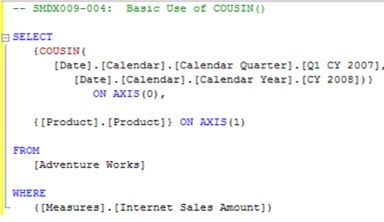
Illustration 13: The Query in the Query Pane

Here, we’re specifying Internet Sales Amount within the slicer specification (WHERE). We are also using the Cousin() function with an ancestor member expression of [Date].[Calendar].[Calendar Year].[CY 2008]. Because we specify the Year level, with Q1 CY 2007 as the source member, we would expect to see the first quarter for calendar year 2008 in the result dataset. We will not be disappointed in our expectations.

Click the Execute (!) button in the toolbar.

Analysis Services populates he Results pane.

Illustration 14: The Dataset Returned Employing the Cousins() Function

The results dataset displays the total at the level of the quarter of Q1 CY 2008, the cousin of the source quarter Q1 CY 2008.

Save the query by selecting File Save MDXQuery3.mdx As …, naming the file SMDX009-004.mdx.

Now let’s illustrate the operation of the Cousin() function once again, with another example. This time, we will write a query to return total Internet Order Quantity for the three child months of Calendar Year 2007, for customers in the United States of America. We will employ the .Children function, once again, in conjunction with the Cousin() function to enumerate the three child months as individual columns, as we shall see. We will also employ the .Children function in the ON ROWS specification, to establish a row for each child member of the Touring product line, which we have established as the row axis in earlier queries.

Select File New from the top menu, as before.

Select Query with Current Connection from the cascading menu that appears next, once again.

Type (or copy and paste) the following query into the Query pane:

-- SMDX009-005: COUSIN() with .CHILDREN to Descend Another "Generation"
SELECT
{COUSIN(
[Date].[Calendar].[Calendar Quarter].[Q3 CY 2006],
[Date].[Calendar].[Calendar Year].[CY 2007]).CHILDREN}
ON AXIS(0),
{[Product].[Product Model Lines].[Product Line].[Touring].CHILDREN}
ON AXIS(1)
FROM
[Adventure Works]
WHERE
([Measures].[Internet Order Quantity],
[Customer].[Customer Geography].[Country].[United States])

Here we’re specifying the Internet Sales Amount measure in our slicer specification (WHERE), together with the qualified name for United States customers. We are also using the Cousin() function with the source member of Q3 CY 2006 in the Calendar hierarchy of the Date dimension. Because we employ the .Children function to create columns for each of the child months of the third quarter of CY 2007 (the “cousin” of Q3 CY 2006), we expect to see July 2007, August 2007 and September 2007 in those columns. Moreover, because we use the .Children function again in the row specification, this time in conjunction with the Touring member of the Product Line level of the Product.Product Model Lines dimension hierarchy, we would expect to see each of the members of the Touring model line listed in the rows of the returned dataset. Again, our expectations will prove to be correct.

The query appears within the Query pane as depicted.

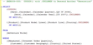
Illustration 15: The Query, Employing Cousin() and .Children

Click the Execute (!) button in the toolbar, once again.

The requested data appears within the Results pane appears:

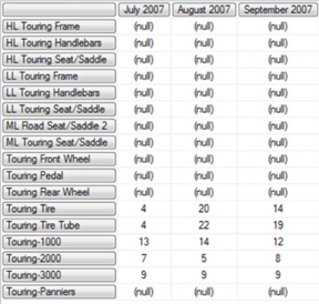
Illustration 16: The Query Results Returned via the Cousin() / .Children Combination

The results dataset displays the total Internet Sales Amounts for United States customers, for each of the members of the Touring product line for months July 2007, August 2007 and September 2007.

Save the query by selecting File Save MDXQuery4.mdx As …, naming the file SMDX009-005.mdx.

All that remains is to take the opportunity, once again, to remove the empty / null cells from the results dataset, as we noted in our similar action earlier, to perhaps make it a bit easier to use for analysis and reporting.

Modify the comment lines (to lines 1 and 2 of the syntax below), and add the keywords NON EMPTY to the far left of the rows specification (line 8) of the query we constructed above, as we have done in earlier queries, as follows:

-- SMDX009-006: COUSIN() with .CHILDREN to Descend Another "Generation"
-- [ADDING "NON EMPTY" TO ROW AXIS TO REMOVE EMPTIES]
SELECT
{COUSIN(
[Date].[Calendar].[Calendar Quarter].[Q3 CY 2006],
[Date].[Calendar].[Calendar Year].[CY 2007]).CHILDREN}
ON AXIS(0),
NON EMPTY {[Product].[Product Model Lines].[Product Line].[Touring].CHILDREN}
ON AXIS(1)
FROM
[Adventure Works]
WHERE
([Measures].[Internet Order Quantity],
[Customer].[Customer Geography].[Country].[United States])

The modified query, with adjusted sections circled, appears within the Query pane as depicted:

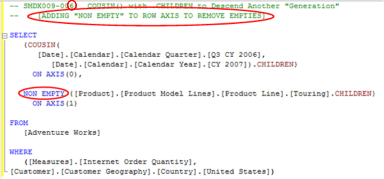
Illustration 17: The Query (with Modifications Circled) in the Query Pane

Press F5 to execute the newly modified query.

Analysis Services returns data to the Results pane:

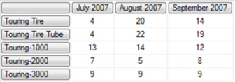
Illustration 18: Results Dataset – Applying Non Empty to Eliminate Nulls

As before, the results dataset displays the Internet Order Quantity totals for the children of the Touring bike product line, for the three months comprising quarter 3 of Calendar Year 2007, as purchased by customers in the United States. But this time the empty intersects are removed. Once again, the NON EMPTY keywords facilitate the suppression of empties, and the removal of any tuples on the affected axis that are associated with empty intersects.

Save the query by selecting File Save SMDX009-005.mdx As …, naming the file SMDX009-006.mdx.

Exit SQL Server Management Studio as desired.

As I noted in Level 5: Members, and an Introduction to the MDX Members Functions , we will call upon the “family” functions we have examined in this Level frequently, as we move into subsequent steps’ coverage of many of the functions available in MDX, as well as into progressively more advanced stages of query building. Moreover, as I have stated throughout the Stairway to MDX series so far, a grasp of the basic operators and functions will be vital to success in our taking advantage of the more complex MDX concepts that we will uncover as we proceed. Practice with these components will assure that their use comes as second nature, and will create a foundation from which the power and elegance of MDX can be fully exploited.

Summary …

In this Level, we concluded the introduction to the MDX “family” member functions we began in Level 5: Members, and an Introduction to the MDX Members Functions. In this Level, we focused upon the .LastSibling and Cousin() functions, discussing for each the syntax within which it is employed, as well as the information it returns and other details. We gained the know-how needed to take advantage of these useful functions through the typical Stairway practice exercises, whereby we constructed queries that used each function, and then examined the results datasets those queries delivered.