The Order() function provides the 'hierarchized' sorts you need for reports and applications using MDX. In this Level, Business Intelligence Architect Bill Pearson explores using the versatile Order() function for providing dataset sorts that respect dimensional hierarchies.
In this session, we’ll introduce a basic function that finds itself within expressions and queries that rank, in terms of sophistication, from the simplest to the most advanced. The Order() function provides sorting capabilities that allow us to reach beyond the natural cube structure, and is therefore an important member of our analysis and reporting toolsets.
As simple as mere ordering might appear to be, the support of hierarchies in MDX makes the processes a bit more involved. Because of the hierarchical nature of Analysis Services cubes, two general types of ordering can be found: ordering within the hierarchy ('hierarchized'), where we want to sort within the existing structure, or no ordering within the hierarchy ('non-hierarchized'), where we wish to ignore (or “break”) that structure. Ordering in a hierarchized manner arranges members within a given hierarchy, and then arranges the hierarchical levels. Without any explicit ordering within the hierarchy ('non-hierarchized') the arrangement of all members within the affected set ignores the hierarchy completely.
In this article, we will examine the use of Order() to perform ordering within the hierarchy. (We’ll look at performing 'nonhierarchized') sorting in our next article.) Whether we set about meeting business analysis and reporting needs by ordering within existing hierarchies, or by ignoring those hierarchies to achieve differing orders, the general purpose of the Order() function is the same: to impose a sort order on a standard MDX set in a manner that allows us to list results based upon some criterion. The Order() function allows us to meet many common and uncommon business needs, including the obvious need to order lists of members within a set, be they employees, products, accounts, customers, months, or others; we might also wish to organize a set of members by specific attributes, such as statuses, degree of completion or readiness, and locations, to name a very few.
The only difference in the use of the Order() functions to provide different types of sorts is the optional order specification at the end of the function, as we shall see.
Order() can accept either a string expression or a numeric expression as criterion for ranking. Syntactically, the sort criteria and the order specification (ASC, DESC, BASC, or BDESC) are placed within the parentheses to the right of Order(), as shown in the following illustration:
Order («Set», {«String Expression» | «Numeric Expression»} [, ASC | DESC | BASC | BDESC])
The Order() function returns hierarchized data (our focus in this article) when the ASC or DESC order specifications are appended to the function, and nonhierarchized data (which we examine in The Order() Function: Beyond Cube Hierarchies)when BASC or BDESC are used. (The “B” serves as an instruction to “break,” or “ignore” the hierarchy.) ASC is the default order specification when none is specified in the function.
In the case of the hierarchized order option, members are first ranked according to position within the hierarchy, then according to each level involved, based upon a string or numeric expression we provide.
The following example expression illustrates a use of the Order() function with the hierarchized order option (inherent with the use of ASC or DESC):
ORDER(
{[Product].[Product Categories].[Category].[Bikes].CHILDREN,
[Product].[Product Categories].[Category].[Clothing].CHILDREN},
[Measures].[Internet Sales Amount], ASC)
This expression, contained within the row specification of a proper query (assuming the specification of the Internet Sales Amount measure in the columns axis), would result in the return of the set depicted in Table 1.
| Internet Sales Amount | |
| Socks | $5,106.32 |
| Caps | $19,688.10 |
| Gloves | $35,020.70 |
| Vests | $35,687.00 |
| Shorts | $71,319.81 |
| Jerseys | $172,950.68 |
| Touring Bikes | $3,844,801.05 |
| Mountain Bikes | $9,952,759.56 |
| Road Bikes | $14,520,584.04 |
Table 1: Ordering of the Set, Hierarchized
Ascending, by Internet Sales Amount
In the expression above, we use the Order() function to return the contents of the Bike and Clothing product categories, in Ascending (ASC) order, with respect to the total Internet Sales Amount for each. Because we use ASC (and therefore the hierarchized option), we order with respect to the existing hierarchy: We obtain the Clothing children first, sorted by Internet Sales Amount in ascending order, followed by the children of the Bikes category, sorted in ascending order. Note that, even though we specify the Bikes category before the Clothing category in the set we specify, Clothing precedes Bikes in the returned dataset. This is again because the expression we have rendered results in ordering within the existing hierarchy of the Product dimension. So we end up with an ascending sort for the children within the two categories we specify, and then a sort of those categories themselves, based upon total by Internet Sales Amount.
We can order the result dataset based upon any relevant measure in just this fashion. Needless to say, proper selection, as well as filtering, of dimensions and levels is critical to prevent the MDX query from returning unexpected results.
Let’s get some hands-on exposure to the basics. We’ll begin with a basic query, in the practice steps that follow, which does not order the data it retrieves, but returns it in its “natural” order. We will then have a frame of reference from which to get some practice with sorting the same data within the hierarchical structure of a representative dimension.
Using the Order() Function to Generate Hierarchized Data
Let’s reinforce our understanding of the basics we have covered so far, by using the Order() function in a manner that illustrates its operation in returning hierarchized data, one of the two general, order-type options that are available, as we mentioned earlier. We will rely upon the SQL Server Management Studio (“SSMS”), once again, as our tool for constructing and executing the MDX we examine, and for viewing the result datasets we obtain. (If you are not sure how to set up SSMS to access the Adventure Works DW 2008R2 database, then click here for a guide.)
- Start SSMS.
- Connect with the appropriate Analysis Server, and select the Adventure Works cube within the Adventure Works DW 2008R2 database from the Object Explorer.
- Click the New Query button just above the Object Explorer to open a blank Query pane, ensuring that Adventure Works appears in the Cube selector atop the Metadata pane to the right of the Object Explorer.
“Natural Order” within a Dimension
We will begin our exploration of the Order() function by examining how a set of data looks “unordered.” As we noted earlier, this will establish a frame of reference upon which we can build an understanding of how Order() can be used to sort. As many of us know, “natural” ordering within a given dimension of a cube is driven by the OrderBy property setting for the respective dimension attribute. It is important to keep in mind that sorting by measures is not “natural,” and must be accomplished via the Order() function, or by some other means, within MDX.
-- SMDX003-001 Simple, unordered dataset, to demonstrate
-- default, "natural" sort, based upon OrderBy property
-- of respective attribute
SELECT
{[Measures].[Reseller Sales Amount]} ON AXIS(0) ,
{[Geography].[Geography].[Country]} ON AXIS(1)
FROM
[Adventure Works]
The Query pane appears, with our input.

Illustration 1: Our Initial Query in the Query Pane …

Illustration 2: Click Execute to Run the Query…
The Results pane is populated by Analysis Services, and the dataset appears.
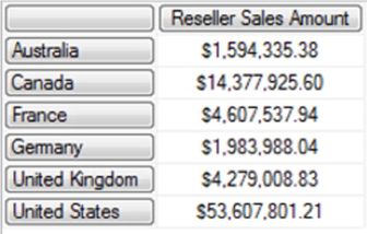
Illustration 3: Results Dataset
– “Natural” Ordering
In the returned dataset, we see that the data is ordered by the Country names. This “natural order” is enforced by the OrderBy setting within the Country dimension attribute properties, which we can examine within the Business Intelligence Development Studio, where “Name” is selected as shown:
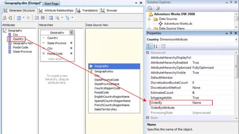
Illustration 4: OrderBy Attribute Property Setting is “Name”
It’s easy, then, to see that the “natural” sort order, which is driven by an attribute property setting, has nothing to do with the measure we have specified within the column axis of our query. For that matter, as we have intimated, the only way that we can sort by a measure is through a method outside the physical dimensional structure. Order() provides the means to do this, as we shall see in our next query.
- Type (or cut and paste) the following query into the Query pane:
- Execute the query by clicking the Execute button in the toolbar...
- Select File --Save MDXQuery1.mdx As …, name the file SMDX003-001, and place it in a meaningful location.
Using the Order() Function to Sort Our Data
Let’s start with a simple query to gain an understanding of the use of the Order() function to return hierarchized data, or data sorted within hierarchical considerations. Our query will focus on Reseller Sales Amount, a value that is captured monthly within the Adventure Works organization, and which is stored in the Adventure Works cube. We will begin with a core query that simply pulls unsorted data, and then add Order() to achieve a desired result.

Illustration 5: Create a New Query with the Current Connection …
A new tab, with a connection to the Adventure Works cube (we can see it listed in the selector of the Metadata pane, once again) appears in the Query pane.
-- SMDX003-002 Simple, starter dataset, "natural" sort
SELECT
{[Measures].[Reseller Sales Amount]} ON AXIS(0) ,
NON EMPTY
{[Geography].[Geography].[State-Province].[Alabama].CHILDREN,
[Geography].[Geography].[State-Province].[Alabama].CHILDREN}
ON AXIS(1)
FROM
[Adventure Works]
The query also accomplishes a complementary objective: By selecting two separate members of the State-Province level in the Geography dimension to populate the row axis in the query, we have constructed a scenario whereby we know that we have two separate hierarchical levels; we thus have a basis for confirming the real effects of using each of the hierarchical (and nonhierarchical in our next article) sort types.
The Query pane appears, with our input:

Illustration 6: Our Second Query in the Query Pane …
The Results pane is, once again, populated by Analysis Services. The dataset depicted appears:
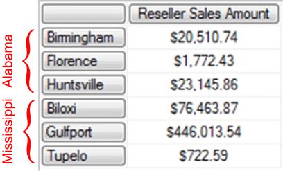
Illustration 7: Results Dataset: Unordered, Retaining “Natural” Hierarchy
We see the total Reseller Sales Amount for each of the specified states returned. Because we have left ordering as it “naturally” occurs in the cube, we see the states of Alabama and Mississippi ordered by Name (“ascending” is the default), and, within that order, we see the cities of each state ordered by name, as well. Reseller Sales Amount is, of course, ignored. This demonstrates, once again, that hierarchical order is enforced.
Let’s employ Order() to work within the Geography hierarchy (State-Province level) of the cube, while ordering the returned data by the measure Reseller Sales Amount.
Another new tab, again connected to the Adventure Works cube, appears in the Query pane.
-- SMDX003-003 Simple use of Order() function, sort descending
-- (respecting hierarchies)
SELECT
{[Measures].[Reseller Sales Amount]} ON AXIS(0) ,
NON EMPTY
ORDER(
{[Geography].[Geography].[State-Province].[Alabama].CHILDREN,
[Geography].[Geography].[State-Province].[Mississippi].CHILDREN},
[Measures].[Reseller Sales Amount], DESC
) ON AXIS(1)
FROM
[Adventure Works]
The query recreates the same scenario we established earlier: it generates two hierarchical levels within which we can confirm our understanding of the Order() function – from a hierarchical perspective. This time, we use Order() to return the contents of the Alabama and Mississippi members of the State-Province levels of the Geography dimension, in Descending (DESC) order, with respect to the total Reseller Sales Amount for each. Because we use DESC (and therefore the hierarchized option), we order with respect to the existing hierarchy: We obtain the Mississippi children first, sorted by Reseller Sales Amount in descending order, followed by the children of Alabama, also sorted in descending order.
Note that, even though we name the Alabama state-province before the Mississippi state-province in the set we specify, we will expect Mississippi to precede Alabama in the returned dataset. This is, once again, because the rendering expressions drive ordering within the existing hierarchy of the Geography dimension. So we end up with a descending sort for the specified children (Mississippi and Alabama) within the State-Province level we specify, and then a sort of the children within each of those State-Provinces, based upon total (at each level) Reseller Sales Amount. Again, we have constructed a scenario whereby we know that we have two separate hierarchical levels; we thus have a basis for confirming the real effects of using each of the hierarchical (and nonhierarchical in our next article) sort types.
The Query pane appears, with our input:
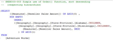
Illustration 8: Third Query: Order() Function (Descending), Respecting Hierarchies
The Results pane is populated, once more, by Analysis Services, and the dataset appears.
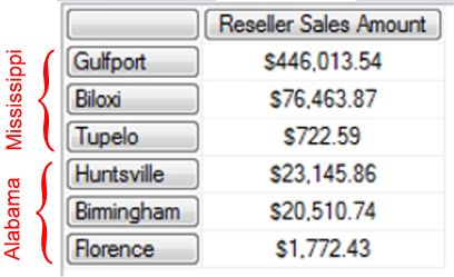
Illustration 9: Results Dataset – Order() Expression in Place, Hierarchized, Descending
As expected,the Order() function sorts our state-provinces (Alabama and Mississippi are specified in the query to populate the row axis) from “highest to lowest,” (and thus “from Mississippi to Alabama”, from the perspective of total Reseller Sales Amount), respecting state groupings in those sorts. We obtain each of the three Mississippi city-children, sorted highest to lowest, with respect to Reseller Sales Amount, followed by each of the three Alabama city-children, also sorted highest to lowest based upon Reseller Sales Amount in descending order.
Finally, let’s take a quick look at how easy it is to generate the same dataset, but this time swapping the columns and rows as we have left them above, and performing our sorts across the columns. The intent here is simply to show that we can perform a columnar sort just as easily as we can do so within the rows of the dataset.
Another new tab, again connected to the Adventure Works cube, appears in the Query pane.
-- SMDX003-004 Simple Use of Order() function across columns,
-- sort descending(respecting hierarchies)
SELECT
NON EMPTY
ORDER(
{[Geography].[Geography].[State-Province].[Alabama].CHILDREN,
[Geography].[Geography].[State-Province].[Mississippi].CHILDREN},
[Measures].[Reseller Sales Amount], DESC
) ON AXIS(0),
{[Measures].[Reseller Sales Amount]} ON AXIS(1)
FROM
[Adventure Works]
The query again recreates the same scenario: it generates two hierarchical levels within which we can confirm our understanding of the Order() function – from a hierarchical perspective. As before, we order with respect to the existing hierarchy: We obtain the Mississippi children first, sorted by Reseller Sales Amount in descending order, followed by the children of Alabama, also sorted in descending order. Moreover, we use Order() to return the contents of the Alabama and Mississippi members of the State-Province levels of the Geography dimension, in Descending (DESC) order, with respect to the total Reseller Sales Amount for each. The difference this time is that we simply swap our column and row specifications to demonstrate a cross-columnar sort
The Query pane appears, with our input:
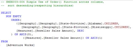
Illustration 10: Fourth Query: Order() Function (Descending), Respecting Hierarchies, Ordering Across Columns
The Results pane is populated, once more, by Analysis Services, and the dataset appears.

Illustration 11: Results Dataset – Order() Expression in Place, Hierarchized, Descending, Ordering Across Columns
As expected,the Order() function sorts our data as before, this time ordering across columns instead of rows, with the total Reseller Sales Amount for each city appearing in the single row of the current dataset.
- Select File -- New from the main menu.
- Select Query with Current Connection from the cascading menu that appears next:
- Type (or cut and paste) the following query into the Query pane:
- Execute the query by clicking the Execute button in the toolbar, as before.
- Select File --Save MDXQuery2.mdx As …, name the file SMDX003-002, and place it in the same location used to store the earlier query.
- Select File --New from the main menu.
- Select Query with Current Connection from the cascading menu that appears next, as we did earlier.
- Type (or cut and paste) the following query into the Query pane:
- Execute the query by clicking the Execute button in the toolbar, once again.
- . Select File -- Save MDXQuery3.mdx As …, name the file SMDX003
- . Select File -- New from the main menu.
- . Select Query with Current Connection from the cascading menu that appears next, as we did earlier.
- . Type (or cut and paste) the following query into the Query pane:
- . Execute the query by clicking the Execute button in the toolbar, once again.
- . Select File -- Save MDXQuery4.mdx As …, name the file SMDX004.
- . Select File -- Exit to leave the SQL Server Management Studio, when ready.
Summary…
In this article, we explored the MDX Order() function, which is found in a range of expressions and queries from the simplest to the most advanced. We learned that Order() provides sorting capabilities that allow us to reach beyond the natural cube structure, and this function is thus an important member of our analysis and reporting toolsets.
We then focused upon the use of the Order() function to return hierarchized data via the appended ASC or DESC order specifications, and looked forward to our next article, The Order() Function: Beyond Cube Hierarchies, where we expose the use of the Order() function to return nonhierarchized data when the BASC or BDESC order specifications are used. Throughout the article, we examined the syntax involved with Order(), and showed some business uses for the function by generating queries that capitalized upon its capabilities.
