To learn MDX, there is really no alternative to installing the system and trying out the statements, and experimenting. William E Pearson, the well-known expert on MDX, kicks off a stairway series on this important topic by getting you running from a standing start.

Contents

Level 1: Getting Started with MDX

MDX, which stands for MultiDimensional eXpressions, is a language with a specialized syntax for querying and manipulating the multidimensional data stored in OLAP cubes. Since it first appeared in Microsoft OLAP Services 7.0 in 1998, a number of other products have adopted it.

In this series, we’ll be getting to the stage of being able to create useful MDX queries in a business context, and we’ll move on from that point to give you a comprehensive understanding of the functions, operators, and properties of MDX.

The objective will be to encourage you to take the example code as you read the ‘levels’, and try it out, making changes and experimenting, so as to get the feel for all the features of MDX. We’ll illustrate every point with practice examples of the business uses along with useful queries. Try them out.

To do this, you need to have installed at least the Analysis Services component of SQL Server 2005 or above. The full installation of SQL Server 2005 and beyond allows for virtually any exercise we might undertake, including occasional references to Reporting Services and other “layers” of the solution – primarily to illustrate the purpose of the queries and the datasets that they retrieve, although the majority of our sessions center on Analysis Services and its underlying components (cubes, dimensions, measures, and such).

For purposes of the series, you should install, or have access to, SQL Server 2008R2, and, specifically, the Analysis Services components of the release (I will often substitute the term “Analysis Services” from now on). You will also need the appropriate access rights to the sample cubes provided in a default installation of Analysis Services.

Installation of Analysis Services from the Standard edition of SQL Server 2008R2 will be adequate for the vast majority of our activities, although the Developer / Enterprise edition is certainly ideal. I will provide references for step-by-step installation of SQL Server 2008R2 Developer / Enterprise in the section that follows.

It is also assumed that the computer(s) involved meet the system requirements, including hardware and operating systems, of the applications we have mentioned.

Installing Analysis Services 2008R2 and Samples

SQL Server 2008 and 2008R2 each provide a virtually identical single Setup program from which you can install any or all of its components, including Analysis Services. Using the unified Setup, you can install Analysis Services with or without other SQL Server components on a single computer. It is important, however, to understand that Analysis Services relies upon other components of SQL Server: for example, the Adventure Works cube (which resides within the Adventure Works DW 2008R2 Analysis Services database), uses the AdventureWorksDW2008R2 relational data mart in SQL Server as its data source, so, if we want to process the Analysis Services database and its cube (we cannot query an unprocessed cube), we will need to have access to its underlying relational data source and, therefore, to SQL Server and the associated sample database.

There are many possible considerations in the installation of Analysis Services, depending upon the version(s) you intend to install, the hardware in your local environment, applications you may already have in place, and so forth. Rather than trying to reproduce them all in this article, we provide the following link, which covers this subject thoroughly, yet efficiently.

Considerations for Installing Analysis Services

Once you have determined the components you need to install, you can follow step-by-step instructions on how to start Setup, and to select the components you want to install, by following this link:

Quick-Start Installation of SQL Server 2008

Once you have successfully installed Analysis Services(along with any other components you have chosen from the Setup program), you are ready to download and install the samples that we will be working with in this series. A great summary of the options that are available (based upon your SQL Server version and other considerations) can be found at:

How to install Adventure Works SQL DW and Analysis Services 2005/2008 sample database and project

Accessing an MDX Editor

We’ll be introducing functions, operators, and other components in a number of sample sessions, using the types of queries that you might come across in your work. I’ll use SQL Server Management Studio to create and execute these queries, so it is easiest to follow what I do with that, although you can certainly use any compatible editor you choose, instead.

To prepare SQL Server Management Studio for writing, modifying and executing MDX queries, and examining the results returned within a practice session, take the following simple steps.

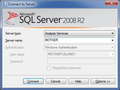
Illustration 2: Connecting to the Server

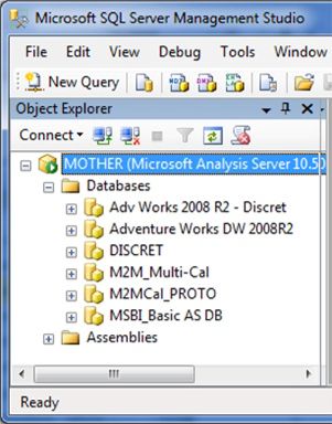
Illustration 3: Exposing the Analysis Services Databases in the Object Browser

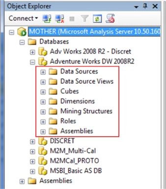
Illustration 4: Exposing the Object Folders in the Database

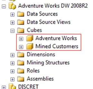
Illustration 5: The Cubes Appear

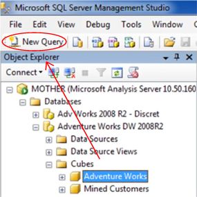
Illustration 6: Click the New Query Button with the Adventure Works Cube Selected

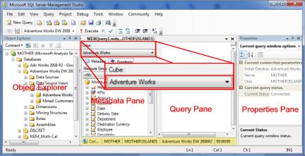
Illustration 7: Adventure Works Cube Metadata Appears

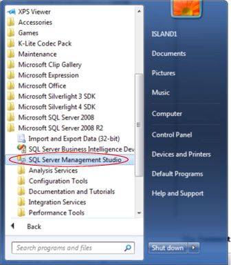
1. 1. Click the Start button on the PC.
   2. Select Microsoft SQL Server 2008 within the Program group of the menu.
   3. Click SQL Server Management Studio, as shown in Illustration 1.

      

      Illustration 1: Opening SQL Server Management Studio

      The Connect to Server dialog appears, after the brief Management Studio splash screen.

   4. Select Analysis Services in the Server type selector
   5. Type / select the server name (server name / instance, if appropriate) in the Server name selector.
   6. Supply authentication information, as required in your own environment.

      The Connect to Server dialog appears similar to that depicted in Illustration 2.

   7. Click the Connect button to connect with the specified Analysis Services server.

The SQL Server Management Studio opens.

1. 1. In the Object Explorer pane (it appears by default on the left side of the Studio), expand the Databases folder (click the “+” sign to its immediate left), appearing underneath the Analysis Server within which we are working.

The Databases folder opens, exposing the detected Analysis Services database(s), as shown in Illustration 3.

1. 1. Expand the Adventure Works DW 2008R2 database.

The Database expands, exposing the folders for the various objects housed within the Analysis Services database, as depicted in Illustration 4.

1. 1. Expand the Cubes folder within the Adventure Works DW 2008 database.

The Cubes folder opens. You may see multiple cubes here, depending upon your local environment. Adventure Works is the sample cube with which I will be conducting the practice exercises. The cubes appear similar to those shown in Illustration 5, within an “out-of-the-box” installation.

1. 1. Click the Adventure Works cube to select it.
   2. Click the New Query button just under the main menu, in the upper left corner of the Management Studio, as depicted in Illustration 6.

The Metadata pane for the Adventure Works cube appears, along with the Query pane to its right, as seen in Illustration 7.

We will be using the Query pane to construct and execute MDX queries throughout the practice sessions of this series.

Creating an MDX query

Introduction

MDX emerged circa 1998, when it first began to appear in commercial applications. MDX was created to query OLAP databases, and has become widely adopted within the realm of analytical applications. Based upon the XML for Analysis (XMLA) specification, with specific extensions for Analysis Services, MDX is the query language that has been specially designed to retrieve multidimensional data, among other activities, in Analysis Services. The components of Multidimensional expressions can be evaluated by Analysis Services to retrieve an object (for example a set or a member), or a scalar value (for example, a string or a number), and consist of identifiers, values, statements, functions, and operators. MDX expressions and queries can be used for numerous activities, including:

• Returning data to a manual editor or client application from an Analysis Services cube;
• Formatting query results;
• Performing cube design tasks, including the definition of calculated members, named sets, scoped assignments, and key performance indicators (KPIs);
• Performing administrative tasks, including dimension and cell security.

You’ll notice, at first blush, that MDX appears similar to the SQL syntax that is typically used with relational databases. Because MDX is not an extension of the SQL language, and is different from SQL in many ways, you’ll need to understand the basic concepts in MDX and dimensional modeling if you intend to work with MDX expressions to design or secure cubes, or to construct MDX queries to return and format multidimensional data. This will include MDX syntax elements, MDX operators, MDX statements, and MDX functions.

Syntax

The basic MDX query contains the SELECT statement: a “SELECT” query is the most frequently used query in MDX. You can gain a good understanding of the use of MDX to query multidimensional data through a grasp of three concepts:

• How an MDX SELECT statement must specify a result set;
• What the syntax of the SELECT statement is; and
• How to create a simple query using the SELECT statement.

Specifying a Result Set

In MDX, the SELECT statement specifies a result set that contains a subset of multidimensional data that has been returned from a cube. To specify a result set, an MDX query must contain the following information:

• The number of axes or sets of hierarchies. (You can specify up to 128 axes in an MDX query, although it is extremely rare to see one with greater than five axes.)
• The members from each dimension to include on each axis of the MDX query.
• The name of the cube that sets the context of the MDX query.
• The members from a slicer axis on which data is sliced for members specified within the query axes.

To identify the query axes, the cube that sets the context of the query, and the slicer axis, the MDX SELECT statement uses the following clauses:

• A SELECT clause - determines the query axes of the SELECT statement.
• A FROM clause - determines which multidimensional data source to use when extracting data to populate the result set of the SELECT statement.
• A WHERE clause (optional) - determines which dimension or member to use as the slicer axis that restricts the extracting of data to a specific dimension or member.

SELECT Statement Syntax

The following syntax shows a basic SELECT statement that includes the use of the SELECT, FROM, and WHERE clauses:

The above shows how the core MDX SELECT statement supports additional, optional syntax, such as the WITH keyword, the use of MDX functions to construct members by calculation for inclusion in an axis or slicer axis, and the ability to return the values of specific cell properties as part of the query.

The following example – much more like the syntax you can expect to encounter in exploring expressions within this series - shows a basic MDX query that uses the SELECT statement. This query returns a result set that contains the calendar years 2006 and 2007 Internet Sales Amount and Internet Order Quantity for the Australian customer base.

In this example, the query defines the following result set information:

• The SELECT clause sets the query axes: Internet Sales Amount and Internet Order Quantity members of the Measures dimension (on columns of the results dataset), and the 2006 and 2007 members of the Date dimension (on rows of the results dataset).
• The FROM clause indicates that the data source is the Adventure Works cube.
• The WHERE clause defines the slicer axis as the Australia member of the Customer dimension (Customer Geography hierarchy).

While the query example uses the COLUMNS and ROWS axis aliases, you can also use the ordinal positions for these axes (as I virtually always do in my articles and in my work with clients). The following example shows how the MDX query could have been written to use the ordinal position of each axis:

Using either of the query examples, you would obtain the results shown in Illustration 8.

Illustration 8: Results of Example Queries

Trying things out: A few initial queries

Procedure: Satisfy Business Requirements with MDX

We will be using SQL Server Management Studio to access the sample Adventure Works cube in the Adventure Works DW 2008 Analysis Services database. I’ve already explained how to get this far. You can create an MDX query, execute it, and see the results in a grid-like results pane.

For purposes of our practice session, assume that you have been given a business requirement by a hypothetical client. You have been asked by a representative information consumer within the client organization (Adventure Works) to provide the total Internet Sales Amounts and Internet Order Quantities, for the years 2006 and 2007 individually, for all customers in the United Kingdom. You are asked, moreover, to provide the information in a two-dimensional grid, with the Internet Sales Amount and Internet Order Quantity measures in the columns, and the calendar years (2006 and 2007) in the rows.

1) Type (or cut and paste) the following query into the Query pane:

When I referenced the Date dimension in the query above, however, I resolved the members uniquely by using their keys. To reference a member by key, you prefix the key with the ampersand (“&”) symbol.

The reason I focus upon this at present is that, when you drag the member from the Metadata tab to the Query pane, instead of simply typing the name, the key is what is inserted on the canvas. Moreover, using the key versus the name means that, even if multiple members have the same name, the member will be resolved uniquely by Analysis Services. (I will use both approaches throughout this series.)

The diagram below labels some of the parts of the query:

Illustration 9: Labeled Parts of a Basic MDX Query

The following general discussion items apply to the syntax above, as well as to MDX queries in general:

• • The top line of the query is a comment. The two dashes (--) represent one of three typical ways to place a comment in MDX syntax, so that it is ignored when the MDX is parsed.

• • The cube that is targeted by the query (the query scope) appears in the FROM clause of the query. The FROM clause in MDX works much as it does in SQL (Structured Query Language), where it stipulates the tables used as sources for the query.

• • The query syntax also uses other keywords that are common in SQL, such as SELECT and WHERE. Even though there are apparent similarities in the two languages, there are also significant differences. A prominent difference is that the output of an MDX query, which uses a cube as a data source, is another cube, whereas the output of an SQL query (which uses a columnar table as a source) is typically columnar.

    It is important to realize that MDX’s cube output allows you to place any dimension from the source cube onto any axis of the query’s result cube. Many axes can exist, and it is often better to think in terms of “axes” than in “dimensions” (as is quite common among both developers and information consumers) when designing an MDX query. This is for two main reasons: The “axes” concept allows for distinction between the source dimensions and the apparent result cube dimensions, which may be very different, indeed. Another reason is that a given axis can contain a number of cube dimensions in combination/juxtaposition. Axis references are therefore more precise, and less subject to misinterpretation.

• • A query has one or more axes. The query we constructed above has two. (The first three axes - ordinals 0 through 2 - that are found in MDX queries are known as columns, rows and pages.) We stipulated the axes above through our use of the “columns” and “rows” specifications. (We could also have done so via the axis ordinals, as I mentioned earlier, in the introduction – we will use ordinals in the next example, and then in most examples going forward in this series). Keep in mind that columns always come before rows, and rows always precede pages, within the query.

• • Curled brackets ( “{ }” ) are used in MDX to represent a set of members of a dimension or group of dimensions. The simple query above has one dimension each on the two query axes. The dimensions that appear are the Measures and Date dimensions.

• • You can display more than one dimension on a result axis. When you do this, an “intersection” occurs, in effect, and each cell appearing in the associated axis relates to the combination/ juxtaposition of a member from each of the indicated dimensions. When more than one dimension is mapped onto an axis, the axis is said to consist of “tuples,” containing the members of each of the mapped dimensions.

• Dimensions that are not specified within the axes of a query will have members specified by default; you can also stipulate such members in the WHERE clause, as shown in our query above.

2) Click the Execute (!) button just underneath the main menu (and above and to the right of the Object Explorer, assuming it is anchored in its default location on your local system), as shown in Illustration 10.

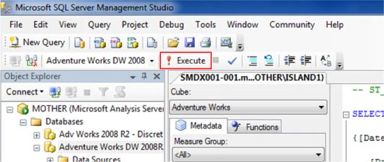
Illustration 10: Click the Execute (!) Button

The retrieved data appears on the Results tab, underneath the Query pane, as soon as Analysis Services fills the cells that it determines to be specified by the query. Your results should appear as depicted in Illustration 11.

Illustration 11: The Initial Query Results

3) Save the query by selecting File à Save MDXQuery1.mdx (or similar name) As …, and call the file SMDX001, as shown in Illustration 12.

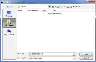
Illustration 12: Saving the MDX Query via the Save As Dialog

Let's create another query to conclude this introductory session. This time, let’s say that client information consumers have asked for a comparison between the total Reseller Sales for the first and second quarters of calendar year 2007. We will again create a query against the Adventure Works cube to generate this information.

4) Select File à New from the main menu.

5) Select Query with Current Connection from the cascading menu that appears next, as depicted in Illustration 13.

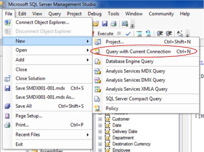
Illustration 13: Create a New Query with the Current Connection

A new tab, with a connection to the Adventure Works cube (you can see it listed in the selector of the Metadata pane, as expected) appears in the Query pane.

6) Type (or cut and paste) the following query into the Query pane:

The Query pane appears, with our input, as shown in Illustration 14.

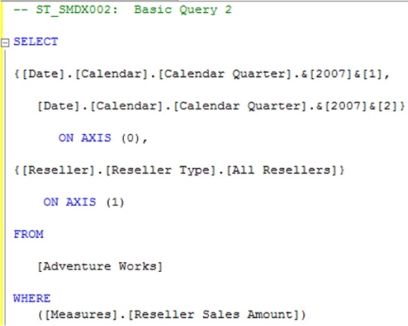
Illustration 14: Our Second Query in the Query Pane

7) Execute the query by clicking the Execute (!) button in the toolbar.

The Results pane is populated by Analysis Services, and the dataset depicted in Illustration 15 appears.

Illustration 15: Results of the Second Query

Because we have specified the Reseller Sales Amount measure in the WHERE statement, we have made it the slicer dimension. The slicer shows that we have picked only the Reseller Sales Amount measure from the measures dimension. We will work with slicer dimensions, as well as with the other components of the simple queries you have examined in this lesson, and far more, as we progress through the Stairway to MDX series.

8) Select File à Save As, name the file ST_SMDX002, and place it with the first query in a meaningful location.

9) Select File -à Exit to leave the SQL Server Management Studio, when ready.

Summary

With this article, I introduced the Stairway to MDX series. I began by noting that the series is designed to provide hands-on introduction to the basics of the Multi-Dimensional eXpressions (MDX) language, with each article progressively exposing an individual function or other component designed to meet specific real-world needs. One of my objectives is to make each lesson as “standalone” as possible, meaning that readers should rarely encounter cases where they cannot complete the practice steps of a given article without components or objects that they have created in previous articles (although I will provide meaningful cross-references, to direct readers to more information about functions and other components I have previously explored, and which the readers may be using in the context of the article at hand).