In the charter Level of this series, Getting Started with PowerPivot and DAX, we introduced the powerful PowerPivot / DAX combination, noting that this add-on to Microsoft Office Excel 2010 insulates Excel users from many of the complexities of other components of the integrated Microsoft BI solution. By leveraging the largely intuitive DAX functions, knowledgeable developers and information consumers will be able to rapidly extract and present the information needed to support enterprise decision makers in a timely, reliable manner. We further noted that we can enjoy high-speed lookups and calculations via an in-memory engine that DAX is designed to leverage in an optimal manner, when working with columns and tables in relational data sources.
We stated in Level 1 that the primary objective of the Stairway to PowerPivot and DAX series is to help readers become comfortable with creating useful queries, within a business context, using PowerPivot and DAX. The goal, we further noted, is to construct formulas from the DAX functions that we introduce within the Levels of this Stairways series, explaining that, for each function we introduce, we will discuss its purpose, the syntax with which it is employed, and the data that it retrieves and presents, all within the context of practice examples of business needs that we address with practical solutions. We encouraged readers to take the example code accompanying each of the ‘Levels’, and to try it out while reading the article, making changes and experimenting, so as to get the feel for the capabilities of PowerPivot and DAX.
In this Level, we expose the COUNTROWS() and FILTER() functions, which, as we shall see, work well in tandem to enable us to perform a count upon a filtered table. The general purpose of COUNTROWS() is simply to return a count of rows in a table we specify or define through an expression. The FILTER() function, in its simplest form, returns a subset of another table / table expression. We’ll discuss ways in which each of these functions can be employed, first in a standalone example for COUNTROWS(), and then in a situation where we employ them together, to achieve a result similar to something we might need to generate for clients or employers in our own environments. As part of our discussion, for each of COUNTROWS() and FILTER() we will:
- Examine the syntax surrounding the function;
- Undertake illustrative examples of the uses of the function in practice exercises;
- Briefly discuss the results datasets we obtain in the practice examples.
In addition to introducing these two new DAX functions, we will examine the output we obtain via calculated columns we construct within the Power Pivot window in the section that follows. We will further create calculated measures, within a new PivotTable, that use the COUNTROWS() and FILTER() functions to replicate the behavior that we have examined in the calculated columns created in the PowerPivot window. We will compare and contrast calculated columns and calculated members in general, and discuss criteria to consider in choosing which of these calculation types to use to meet requirements we encounter in supporting employers and clients.
Preparation for the Levels of the Stairway to PowerPivot and DAX Series
As we’ll note throughout, to obtain the most benefit from the Levels of the Stairway to PowerPivot and DAX series, you will need to have installed the PowerPivot for Excel 2010 add-on on your machine. You will also need to have installed SQL Server 2008 / 2008R2 (including Analysis Services) and the respective relational and Analysis Services samples on your local machine, or have the client portions of each on your machine with access to the rest on a server. To perform all steps of preparation, see the installation section of the charter Level of this series, Step 1: Getting Started with PowerPivot and DAX.
Preparation for the Practice Exercises in this Level
Once we’ve got the PowerPivot for Excel 2010 add-in, SQL Server 2008R2 and the samples noted above installed, we’re ready to perform the practice exercises within this Level. Importing the sample database and taking other preparatory steps are key to providing the environment required to successfully complete this Level, and should be performed before beginning. Because we will work with different data sources throughout this series, the steps of environment preparation will be repeated in various steps. The objective is to make each Level a freestanding session that can be completed independently of other Levels, so that you can focus upon meeting your own immediate requirements efficiently. Where appropriate, references to functions, procedures and other details will be supplied, but the idea of each Level is to focus upon one or more specific DAX functions and / or PowerPivot procedures to satisfy needs that mirror requirements we encounter in our own business environments.
Let’s open PowerPivot and import our data by taking the steps below. This will put us in position to begin learning the material in this Level.
- From the Start menu, select Microsoft Excel 2010.
- Above the Excel ribbon, click the PowerPivot tab, as shown.
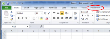
Illustration 1: Click the PowerPivot Tab…
The PowerPivot ribbon appears.
- Click the PowerPivot Window button, appearing at the left of the newly appearing PowerPivot toolbar, as shown.

Illustration 2: The PowerPivot Window Button on the PowerPivot Ribbon…
The PowerPivot window, containing its own ribbon, opens atop the existing Excel spreadsheet, assuming the name of the workbook as its own name, as depicted below.
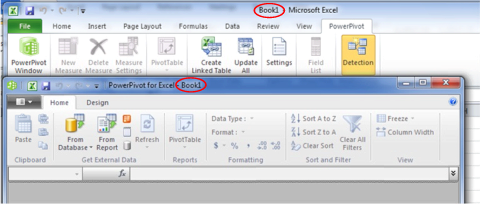
Illustration 3: The PowerPivot Window, Associated with the Workbook, Appears
As we noted in Level 1: Getting Started with PowerPivot and DAX, it is in the PowerPivot window that we load and prepare the data with which we will be working (or will continue working, if data is already added to the workbook). We will typically build a relational model here (even when we import other-than-relational sources, such as Analysis Services data, text files, .RSS feeds, and so forth). As we noted in Level 1, the PowerPivot window displays the tables on individual, tabbed sheets, and is the central place where we import tables, create relationships, maintain column data types and formats, and view, as needed, the data that underlies our data model, among other actions.
Next, we’ll designate a source from which to import data.
- Click the From Database button on the Home tab of the PowerPivot window.
- Select From SQL Server on the drop-down menu that appears next.
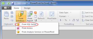
Illustration 4: Select “From SQL Server” in the From Database Dropdown
The Table Import Wizard dialog opens next.
- In the top input box, titled Friendly connection name, type (or copy and paste) the following:
AdventureWorksDW2008R2
- Click the selector (downward pointing arrow) on the right side of the box titled Server name.
PowerPivot begins a scan of the machine to detect, and return to the selector, the available server choices.
- Select the appropriate server for your local environment, or type in the server name / localhost, as appropriate.
- Enter the authentication as required for the local environment (ideally selecting Use Windows Authentication).
- Select AdventureWorksDW2008R2 using the dropdown selector to the right of the box titled, Database name, at the bottom of the dialog.
The Table Import Wizard dialog, with our input, appears similar to that depicted below.
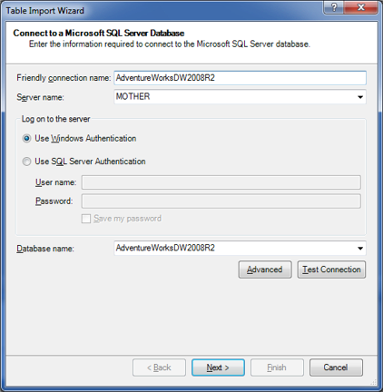
Illustration 5: The Table Import Wizard Dialog, with Our Input
- Click the Test Connection button underneath the Database name selector.
A message box appears, indicating that the test connection has succeeded.

Illustration 6: “Test Connection Succeeded”
- Click OK to dismiss the message box.
- Click the Next button at the bottom of the Table Import Wizard dialog.
- On the dialog that appears next, labeled Choose How to Import the Data, leave the radio button at its default of Select from a list of tables and views to choose the data to import, as shown.
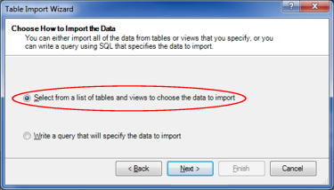
Illustration 7: Choose “Select from a list of tables…” Option for Data Import
- Click the Next button.
PowerPivot loads the tables and views from the AdventureWorksDW2008R2 database into the Select Tables and Views page of the Table Import Wizard that appears next.
- Select the following tables, by clicking the checkbox to the immediate left of the respective table listing in the dialog:
- DimCurrency
- DimCustomer
- DimDate
- DimProduct
- DimProductCategory
- DimProductSubcategory
- DimPromotion
- DimSalesTerritory
- FactInternetSales
The Select Tables and Views dialog appears, as partially shown, with our selection and related tables checked.
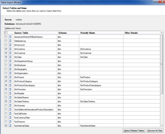
Illustration 8: Selecting Tables (Partial View)…
The idea in these immediate steps is to import enough information into our model to allow us to do some illustrative analysis surrounding the business activities conducted by our hypothetical client, the Adventure Works organization.
- Click the Finish button.
The import process runs, and then we see a “Success” message, complete with a Details list that indicates population by our choices.
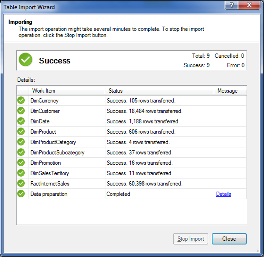
Illustration 9: Success is Indicated, Along with a List of Tables Imported
- Click Close.
The Table Import Wizard is dismissed, and we arrive at the PowerPivot window once again, where we see the imported data as partially depicted.
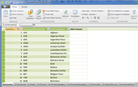
Illustration 10: Imported Data, with a Tab for Each Table
Note that a tab for each imported table has been created in the PowerPivot window (the tabs appear in the bottom left of the window, as seen above). What we are now seeing is not an Excel table, but a view of the efficiently compressed columnar database that PowerPivot uses to store imported tables in memory. For more detailed information about the PowerPivot window itself, please see Level 1: Getting Started with PowerPivot and DAX.
- Click the selector underneath the Quick Access Toolbar (assuming it is in the default, above-the-ribbon position), and to the immediate left of the Home tab in the ribbon.
- Select Save As from the dropdown menu that appears, as shown in Illustration 11.

Illustration 11: Select Save As from the Selector within the PowerPivot Window…
- Save the worksheet as ST_DAX02-1.xlsx, placing it in a convenient location.
- Leave the PowerPivot Window open for the practice session below.
We are ready, at this stage, to get some hands-on exposure to two more DAX functions, COUNTROWS() and FILTER(), while continuing to build experience with the general use of PowerPivot to meet business requirements, in the sections that follow.
The COUNTROWS() Function
Introduction
According to the PowerPivot Help for SQL Server 2008R2, the DAX COUNTROWS() function “counts the number of rows in the specified table, or in a table defined by an expression.” COUNTROWS() is a member of the Statistical Functions group, which is composed of functions that aggregate data and return a scalar value. Statistical functions typically operate upon all rows of a table housing the column that is specified within the function.
COUNTROWS() is highly useful in numerous contexts, particularly when used in conjunction with other functions. An example of a common case, which we’ll see in action later in this Level, is a situation where it provides, in combination with the DAX FILTER() function, a means of counting rows within a filtered table.
We will examine the syntax for the COUNTROWS() function after a brief discussion in the next section. We will then explore its use, including some of the “logic leverage” it offers the knowledgeable user, within practice examples constructed to support hypothetical business needs. This will allow us to activate what we explore in the Discussion and Syntax sections, where we will get some hands-on exposure in creating calculations that employ the COUNTROWS() function.
Discussion
To restate our initial explanation of its operation, the COUNTROWS() function, when acting upon a specified table name, or an expression that returns a table, counts and returns the number of rows in the table / table expression. COUNTROWS() returns a number. The COUNTROWS() function can be used to simply count and return the number of rows in a base table, but, more typically, is employed to count and return the number of rows resulting from applying context to, or filtering, a table.
COUNTROWS() returns a blank when there are no rows to count in the table specified within the function. In contrast, COUNTROWS() returns a zero (“0”) when rows are present within the specified table, but none of these rows fit the specified criteria.
Let’s look at some syntax illustrations to further clarify the operation of COUNTROWS().
Syntax
Syntactically, in using the COUNTROWS() function to return the associated row count number, the table / table expression upon which we seek to apply the function is specified, within parentheses, to the right of COUNTROWS(). The general syntax is shown in the following string:
COUNTROWS(<table>)
Putting COUNTROWS() to work is straightforward. When using the function to return the row count number of the table / table expression (“<table>” in the syntax string above) with which it works, we simply enclose the table name or expression in parentheses to the right of the COUNTROWS() keyword, as we have noted. For example, we might add a column to the DimProductCategory tab of the PowerPivot window, where we have performed the imports described in the Preparation section above, using COUNTROWS() as follows:
=COUNTROWS(DimProductCategory)
The calculated column would return 4, the number of rows in the DimProductCategory table.
As is probably obvious, the COUNTROWS() function can be best leveraged by combining it with other DAX functions, as we shall see in short order.
We will get some hands-on practice with the COUNTROWS() function in the section that follows.
Practice
To reinforce our understanding of the basics we have covered so far, we will use the COUNTROWS() function to define a couple of calculations. We will revisit its use in combination with the FILTER() function when we examine that function in a later section – for now, we just want to understand the basics. The intent, as in all the practice sessions of the Stairway to PowerPivot and DAX series, is to demonstrate the operation of each of the functions we examine in a straightforward, memorable manner.
We will turn to the Excel worksheet we prepared earlier as a platform from which to construct and execute the DAX we examine, and to view the results we obtain.
- Return to the worksheet we created in the Preparation for the Practice Exercises in this Level section above, ensuring that the PowerPivot Window is open, where we left it earlier.
- Click the DimProductSubcategory tab.

Illustration 12: Click the DimProductSubcategory Tab…
- Click the top row in the column labeled “Add Column,” which appears on the far right side of the tab, as shown.
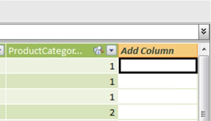
Illustration 13: Click the Top Row in the Column Labeled “Add Column”
- Select the function button (“fx”) to the left of the formula bar next.
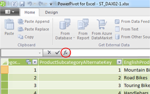
Illustration 14: Select the Function (fx) Button…
The Insert Function dialog appears.
- Click the downward pointing arrow on the selector appearing atop the dialog under the Select a category label.
The following DAX function categories appear:
- All
- Date & Time
- Math & Trig
- Statistical
- Text
- Logical
- Filter
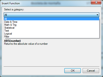
Illustration 15: Insert Function Dialog with Expanded Category Selector
- Select the Statistical category.
- In the Select a function list that populates for the Statistical category, select the COUNTROWS() function, as shown in Illustration 16.
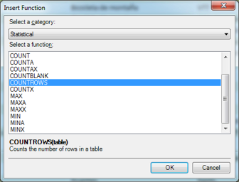
Illustration 16: Select the COUNTROWS() Function
- Click OK to confirm the selection and dismiss the Insert Function dialog.
The COUNTROWS keyword, preceded by the “=” operator and followed by a left parenthesis ( “(“ ) appears in the formula bar, with a function usage tooltip appearing just underneath the function.

Illustration 17: The Beginning of the COUNTROWS() Function, along with Tooltip, Appears
- Because we know that we need now to add the appropriate table name / expression, begin to type in “DimProductSubcategory.”
As we begin to type the table name, we note that AutoComplete immediately presents us with a list of functions and tables from which to select, as shown.
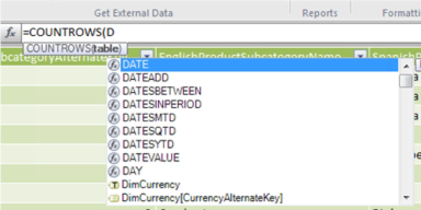
Illustration 18: Functions / Tables as Suggested by AutoComplete…
- Scroll to DimProductSubcategory, and click to select it, as depicted in Illustration 19.
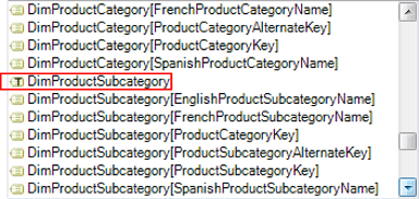
Illustration 19: Select the DimProductSubcategory Table …
Note that the table label, arranged amid various table column labels in the selector list, is preceded by a similar icon to that of the columns, except that it contains a “T” to designate the selection as a table.
- Once the selector is dismissed, and =COUNTROWS(DimProductSubcategory appears in the formula bar, type in a closing right parenthesis ( “)“ ) to complete the formula.
The completed formula appears.
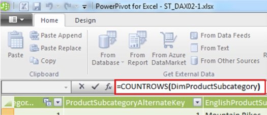
Illustration 20: The Completed Formula Appears
- Press the Enter key.
The column updates and the formula results appear in each row of the new calculated column (the number 37), as partially shown below.
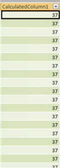
Illustration 21: The Results Appear in Each Row of the New Column (Partial View)
- Right-click the new column header label (currently at its default of “CalculatedColumn1”), and select Rename Column from the cascading menu that appears.
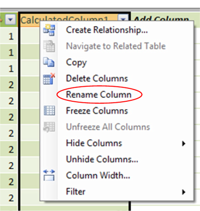
Illustration 22: Renaming the Column to a More Useful Name
- Name the newly added column “No Rows”.
Now let’s construct another calculation involving the COUNTROWS() function, just to reinforce our understanding of its operation under basic conditions. This time, we will employ the function on a different tab of the PowerPivot window.
- Click the DimSalesTerritory tab to transit there.
- Within the DimSalesTerritory tab, click the top row in the column labeled “Add Column,” which appears to the far right of all populated columns, as shown.

Illustration 23: Click the Top Row in the Column Labeled “Add Column,” Once Again
- Select the function button (“fx”) to the left of the formula bar, as we did earlier.
The Insert Function dialog appears, once again.
- Click the downward pointing arrow on the selector appearing atop the dialog under the Select a category label, once again.
- Select the Statistical category within the expanded category selector atop the Insert Function dialog, just as we did in the earlier exercise.
- Select the COUNTROWS() function, once again.
- Click OK to confirm the selection and dismiss the Insert Function dialog.
The COUNTROWS keyword, preceded by the “=” operator and followed by a left parenthesis, once again, appears in the formula bar.
- Begin to type in “DimSalesTerritory.”
As we begin to type the table name, AutoComplete again immediately presents us with a list of functions and tables from which to select.
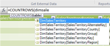
Illustration 24: Functions / Tables as Suggested by AutoComplete…
- Click DimSalesTerritory, to ensure its selection.
- Once the selector is dismissed, and =COUNTROWS(DimSalesTerritory appears in the formula bar, type in a closing right parenthesis ( “)“ ) to complete the formula, as we did earlier.
The completed formula appears as depicted in Illustration 25.
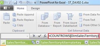
Illustration 25: The Completed Formula Appears, Once Again
- Press the Enter key.
The update occurs, and each row of the new calculated column is populated with the formula results (the number 11), as shown.
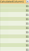
Illustration 26: The Results Appear in Each Row of the New Column
- Right-click the new column header label (currently displaying “CalculatedColumn1,” the default we noted in our first example), and select Rename Column from the cascading menu that appears, as before.
- Name the newly added column “No Rows,” once again.
Having gained familiarity with the COUNTROWS() function within simple usage, we’ll introduce another DAX function, FILTER(), and then return to the COUNTROWS() function to demonstrate the use of COUNTROWS() against an expression wherein we define a filtered table.
The FILTER() Function
Introduction
According to the PowerPivot Help for SQL Server 2008R2, the DAX FILTER() function “returns a table that represents a subset of another table or expression.” FILTER() is a member of the Filter Functions group, which is composed of fourteen functions that specifically support certain advanced types of analysis. Members of the Filter Functions group assist us in navigating tables and iterating over columns to evaluate DAX expressions.
These functions are not “standard” Excel functions.
FILTER() is highly useful in many situations, as it helps us to reduce the number of rows in a table within which we are performing operations, and to narrow down an overall dataset to the specific data we wish to use within a given calculation. FILTER() is not designed to be used in standalone fashion, independent of other functions, but as a function within other functions, as an argument where a table or table expression is required, etc. We’ll see FILTER() in action in this Level of Stairway to PowerPivot and DAX, in a situation where we’ll use it in conjunction with COUNTROWS(), which we introduced in the first half of this Level, to define a table expression whose output is a subset of a larger table.
As we did within our examination of the COUNTROWS() function earlier, we will examine the syntax for the FILTER() function after a brief discussion in the next section. We will then explore its use, including some of the capabilities it offers the knowledgeable user, within practice examples constructed to support hypothetical business needs. This will allow us to activate what we explore in the Discussion and Syntax sections, where we will get some hands-on exposure in creating calculations that employ the FILTER() function.
Discussion
To restate our initial explanation of its operation, the FILTER() function itself returns a table. It is therefore used as an argument, or input, to functions that act upon a specified table / table expression.
Let’s look at some syntax illustrations to further clarify the operation of COUNTROWS().
Syntax
Syntactically, in using the FILTER() function to return a table subset, the table / table expression upon which we seek to apply the function is specified, within parentheses, to the right of the FILTER keyword. The general syntax is shown in the following string:
FILTER(<table>,<filter>)
Putting FILTER() to work is intuitive enough. When using the function to return a table containing only the filtered rows, we simply enclose the table name or expression (comprising the table to be filtered) in parentheses to the right of the FILTER keyword, as we have noted. The filter expression is composed of a Boolean expression that is to be evaluated for each row of the specified table expression (examples might include [Internet Sales Amount] > 1000.00 or [Country] = “Australia”).
An example of FILTER() in use might be as follows:
=COUNTROWS(FILTER(DimSalesTerritory, DimSalesTerritory[SalesTerritoryCountry]="United States"))
The formula returns 5, the number of rows in the DimSalesTerritory table with United States in the SalesTerritoryCountry column.
We will get some hands-on practice with the FILTER() function in the section that follows. We will also use it many times, in conjunction with other DAX functions, throughout the Stairway to PowerPivot and DAX series.
Practice
To gain some practical familiarity with the basics we have covered so far, let’s employ the FILTER() function within some basic calculations. A good way to do this, since FILTER() returns a table and does not lend itself to a simple, standalone calculation in the PowerPivot Window or PivotTable, will be to revisit the use of the COUNTROWS() function, which will, in effect, take the otherwise “table” output of FILTER() and return, instead, a count of the rows within the table that FILTER(), in that instance, returns. This should give us a feel for how FILTER() accomplishes its mission, while providing a memorable example of a fairly typical use. As we’ve noted, we’ll get plenty of exposure to FILTER() in future Levels of this series. This is simply to provide a hands-on example to accompany the conceptual introduction we have made in this Level.
We’ll return to the Excel worksheet with which we have been working in the previous section to proceed with our practice examples.
- Return to the worksheet we created in the Preparation for the Practice Exercises in this Level section above, ensuring that the PowerPivot Window is still open.
- Click the DimSalesTerritory tab.
- Click the top row in the next column labeled “Add Column,” again on the far right side of the tab (to the immediate right of the “No Rows” column we added in the last exercise.
- Select the function button (“fx”) to the left of the formula bar, as we did earlier.
The Insert Function dialog appears, once again.
- Click the downward pointing arrow on the selector appearing atop the dialog under the Select a category label, as before.
- Select the Statistical category, once again.
- Select the COUNTROWS() function, once again.

Illustration 27: Select the COUNTROWS() Function, Once Again
- Click OK to confirm the selection and dismiss the Insert Function dialog.
The COUNTROWS keyword, preceded by the “=” operator and followed by a left parenthesis ( “(“ ) appears in the formula bar, just as it did when we introduced it in the previous section, as shown.
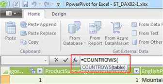
Illustration 28: The COUNTROWS() Function, along with Tooltip, Appears, Once Again
- Type in the letter “F.”
- Via the AutoComplete list that appears, scroll down to the FILTER() function.
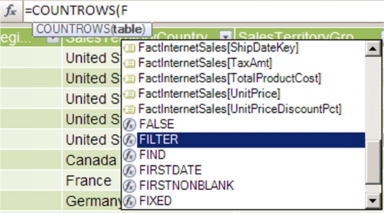
Illustration 29: Scroll to the FILTER() Function within the AutoComplete List
- Click the FILTER() function to select it.
The AutoComplete list is dismissed and the FILTER keyword appears, within the COUNTROWS() function we previously added, in the formula bar, with a left parenthesis ( “(“ ) alongside it, as shown.

Illustration 30: The FILTER() Function “Under Construction” within the Formula Bar
- Because we know that we need now to add the appropriate table name / expression, (we are even reminded of this in the tooltip that appears just under the formula bar), begin to type in “DimSalesTerritory.”
- As the AutoComplete list again appears, scroll to DimSalesTerritory as shown (again, the label is preceded by a “T” icon that designates the selection as a table) and click to select it.
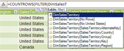
Illustration 31: Select the DimSalesTerritory Table…
- Once the selector is dismissed, and =COUNTROWS(FILTER(DimSalesTerritory appears in the formula bar, type in a comma ( “,“ ) to separate the table expression from the filter argument to be added next.
- Next, begin to type in the DimSalesTerritory table name again, with the intent this time to select the SalesTerritoryCountry column therein.
- Select DimSalesTerritory[SalesTerritoryCountry] in the AutoComplete list.

Illustration 32: Select DimSalesTerritory[SalesTerritoryCountry] in the AutoComplete List
- Once the selector is again dismissed, and =COUNTROWS(FILTER(DimSalesTerritory, DimSalesTerritory[SalesTerritoryCountry] appears in the formula bar, type in an “equals” sign ( “=“ ) to the right of the text appearing in the formula bar.
- Type the following to the immediate right of the “=” sign:
“United States”))
The complete text appears, in the formula bar, as shown.

Illustration 33: The Complete Text in the Formula Bar
- Press the Enter key to generate the contents of the new calculated column.
The new calculated column populates with the number “5,” (the number of rows in the DimSalesTerritory table that contain the phrase “United States” in the SalesTerritoryCountry column).
- Right-click the header for the new calculated column, currently labeled “CalculatedColumn1,” and select Rename Column from the context menu that appears.
- Type the following to rename the column:
No US Rows
The new calculated column appears as shown.
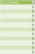
Illustration 34: The Newly Populated “No US Rows” Column
As most of us are aware by now, a distinct strength of PowerPivot environment lies in the fact that the same data and slicers can be shared by multiple PivotTables. Let’s see just how straightforward this is by taking a look, in the section that follows, at a PivotTable example where we can see how to access components with which we have worked so far in this Level of our series. We’ll also look at how to replicate the same logic we employed in the calculated columns we created in this section to create calculated measures in a PivotTable.
Accessing PowerPivot Calculated Columns from a PivotTable and Introducing Calculated Measures
PowerPivot exists, in its most fundamental and common use, to act as a data source for PivotTables. In addition to gaining some exposure to presenting values and calculations from the PowerPivot window within a PivotTable, we’ll overview some basics about PivotTables in general, as well as illustrating a couple of points we need to consider when working with the PowerPivot / PivotTable combination. Specifically, we will
- Expose how to access, and leverage, PowerPivot calculated columns in the PivotTable;
- Discuss PivotTable components, focusing on the nature of measures in the PivotTable;
- Demonstrate how to employ DAX functions in the PivotTable to create calculated measures;
- Explore the differences in calculated columns and calculated measures, particularly within the context of their use within a PivotTable.
We can begin our work with a PivotTable from either the Excel workbook or from the PowerPivot window. Because we’re already in the latter, we will proceed from there by taking the following steps:
- From the DimSalesTerritory tab in the PowerPivot window, click the downward pointing arrow on the PivotTable button to cause the drop-down menu to appear, as shown.
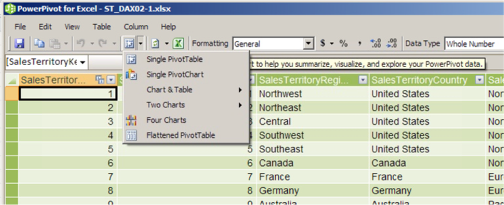
Illustration 35: The PowerPivot Drop-down Menu Appears…
As is obvious from the multiple selections, we can do more than simply assemble a single PivotTable here. While we will work with examples, at various times throughout our series, of some of the other options we see in the dropdown menu (single PivotChart, Chart & Table, Two Charts, Four Charts, and Flattened PivotTable), we will build a single PivotTable in most of the practice sessions of our series, as this will be the most straightforward (and rapid) avenue to getting hands-on exposure to the underlying PowerPivot data and DAX, in general.
- Click Single PivotTable in the dropdown menu we’ve exposed (the tope selection).
We are returned to the Excel window, where we encounter the Create PivotTable dialog.
- Ensure that the radio button labeled New Worksheet is selected.
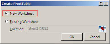
Illustration 36: Ensure the New Worksheet Option is Selected
4. Click OK to accept the setting and dismiss the dialog.
The PivotTable placeholder / canvas, together with the PowerPivot Field List, appear on the new worksheet as depicted (compressed view).
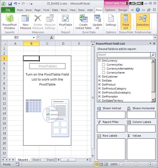
Illustration 37: The PivotTable Canvas Appears on the New Worksheet (Compressed View)
We note that the position of the new PivotTable is set to lie within the range of cell B3 to cell D20. This placement occurs for a reason that will become evident many times in the Stairway to PowerPivot and DAX series: to afford space for the insertion of vertical and horizontal slicer buttons to frame the PivotTable, should we make the selections needed to use them. We also see that the PowerPivot Field List, appearing to the right of the PivotTable, contains elements that will be new to those of us that have become familiar with the standard PivotTable Field Lists: two new, Slicer zones are now included.
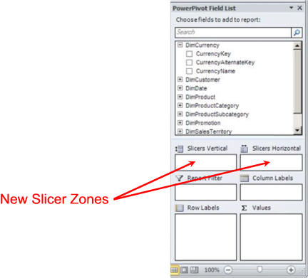
Illustration 38: Two New Slicer Zones Appear in the PowerPivot Field List
Because we’re looking at it for the first time in this Level of the series, and particularly for those not familiar with standard Excel PivotTables, Table 1 below gives a description for each of the areas / zones on the PowerPivot Field List.
PowerPivot Field List Area | Description |
| Search Area | Allows us to perform searches using any part of a field name. (Wildcards are employed on both sides of typed text, by default.) If results are returned for multiple fields, we can move backward or forward through the search results using the left and right arrow buttons, respectively. |
| Slicers Vertical | To filter data by values in a given field, we simply drag the field into this drop zone. The Slicer control appears along the left of the PivotTable when we do so. |
| Slicers Horizontal | To filter data by values in a given field, we simply drag the field into this drop zone. The Slicer control appears atop the PivotTable when we do so. |
| Report Filter | Items we drop into the Report Filter zone filter the entire report by the respective items. When in use, the filter control dropdown list appears immediately above the affected PivotTable or PivotChart. (Example: For a PivotTable report presenting sales for all products, dropping the DimCustomer field from the PivotTable canvas depicted above would enable filtering by members of the Customer dimension.) |
| Column Labels | Allows us to display fields in columns, and supply the field name as the label atop the PivotTable report, like a columns axis. Nesting can be accomplished by dropping the column to be nested below the column within which it is to be nested. |
| Row Labels | Allows us to display fields in rows, and supply the field name as the label on the side of the PivotTable report, like a rows axis. Nesting can be accomplished by dropping the column to be nested below the column within which it is to be nested. |
| Values | Here we select fields (typically numeric, but not always) we wish to display as summary data in the PivotTable report. Moreover, we can include calculated columns and measures, as needed. |
Table 1: Areas of the PowerPivot Field List
All tables included in the PowerPivot window appear in the PowerPivot Field list, as depicted in the close-up view below. Table columns are exposed, intuitively enough, by clicking the “+” sign to the immediate left of the table name to expand it.
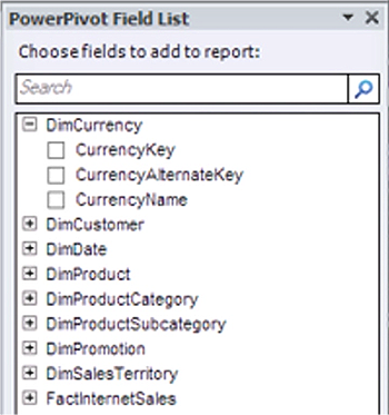
Illustration 39: All Imported Tables Appear, with Columns Only a Click Away…
To gain some exposure to the use of DAX functions within the PivotTable, we will replicate some of the steps we took with regard to one of the tables, DimSalesTerritory, upon which we operated in the PowerPivot window in the earlier part of this Level. In accomplishing this, we’ll see how to approach what we did with the calculated columns earlier, but this time we’ll do so with calculated measures in the PivotTable.
- Expand the DimSalesTerritory table in the Field List by clicking the “+” sign to its immediate left.
The columns of the table, with which we worked in the PowerPivot window in the section above, appear.
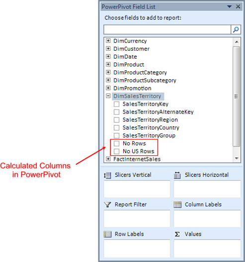
Illustration 40: DimSalesTerritory Table in the PowerPivot Window, Expanded to Show Fields
The last two fields in the expanded list, of course, represent two calculated columns that we created earlier, using DAX functions, in the PowerPivot window. While we could pull these into our new PivotTable like any other field at this point, let’s first examine how to create them as calculated measures – to demonstrate how to use DAX at the PivotTable level.
- Within the PowerPivot Field List, right-click the newly expanded DimSalesTerritory label.
- Select Add New Measure… from the context menu that appears, as shown.
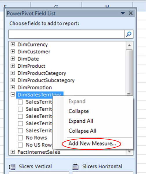
Illustration 41: Select Add New Measure…
The Measure Settings dialog appears.
CM_No Rows
- Type the following into both the Measure Name and Custom Name boxes of the dialog.
- Click the function button (“fx”) to the right of the Formula label, above the Formula box of the dialog.
The Insert Function dialog appears.
- Click the downward pointing arrow on the selector appearing atop the dialog under the Select a category label.
- Select the Statistical category within the expanded category selector atop the Insert Function dialog, just as we did in the earlier exercise.
- Select the COUNTROWS() function, once again.
- Click OK to confirm the selection and dismiss the Insert Function dialog.
The COUNTROWS keyword, preceded by the “=” operator and followed by a left parenthesis, once again, appears in the formula box of the Measure Settings dialog.
- Begin to type in “DimSalesTerritory,” to the right of “COUNTROWS(“ .
As we begin to type the table name, AutoComplete again immediately presents us with a list of functions and tables from which to select, as shown.
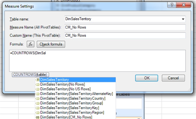
Illustration 42: Functions / Tables as Suggested by AutoComplete …
- Click DimSalesTerritory, to ensure its selection.
- Once the selector is dismissed, and =COUNTROWS(DimSalesTerritory appears in the formula bar, type in a closing right parenthesis ( “)“ ) to complete the formula, as we did for the similar calculated column in the PowerPivot window in the earlier section of this Level.
The completed formula appears as depicted.
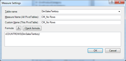
Illustration 43: The Completed Formula Appears in the Measure Settings Dialog
- Click the OK button.
The calculation is saved, and the Measure Settings box is dismissed. The new calculated measure, CM_No Rows, appears in the PowerPivot Field List, underneath the other fields within the expanded DimSalesTerritory fields list. CM_No Rows (we named it this so as to distinguish it from the calculated column No Rows above it) comes “preselected:” the check mark is already in the box to the left of the calculated measure (a calculated measure is indicated by the calculator icon to its immediate right), and the new measure appears, by virtue of its selection, in the Values zone (bottom right corner) of the PowerPivot Field List. Finally, because of its being placed in the Values zone, the calculated measure also appears on the spreadsheet, within the PivotTable, where we see the number “11.” The PivotTable environment appears, reflecting these circumstances, as shown.
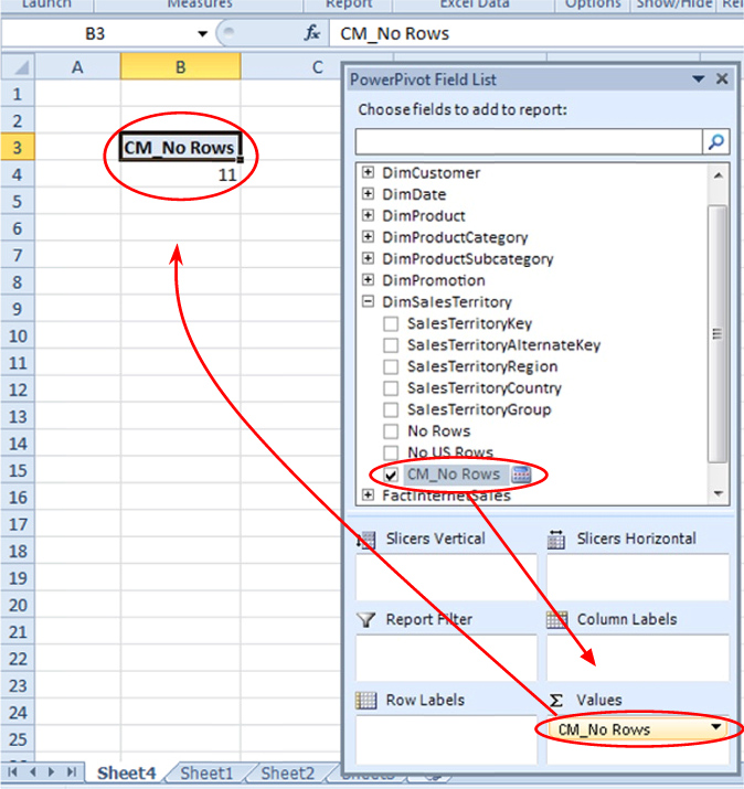
Illustration 44: The PivotTable Environment, Reflecting the Addition of the New Calculated Measure
NOTE: In the above illustration, I have undocked the PowerPivot Field List to allow it to float, and then moved it to the near right of the PivotTable to make displays more concise. To undock, all we need to do is to click the PowerPivot Field List, and, holding down the mouse button, drag the list away from where it originally appears to its desired position. For more information on this, see the Online Help.
Having added a calculated measure to the PowerPivot Field List that is equivalent to what we created as our first PowerPivot calculated column in the earlier section of this Level, let’s add another calculated measure that replicates that logic we used in our second calculated column, No US Rows. Recall that No US Rows also employs the DAX COUNTROWS() function (to again perform a count of the rows in the DimSalesTerritory table), but this time in combination with the FILTER() function (with which we filter the rows counted to include only those relating to the U.S.). We will proceed by taking the following steps:
- Within the PowerPivot Field List, right-click the expanded DimSalesTerritory label, once again.
- Select Add New Measure… from the context menu that appears, as we did before.
The Measure Settings dialog appears, once again.
CM_No US Rows
- Type the following into both the Measure Name and Custom Name boxes of the dialog.
- Click the function button (“fx”) to the right of the Formula label, above the Formula box of the dialog, once more.
The Insert Function dialog appears, as before.
- Click the downward pointing arrow on the selector appearing atop the dialog under the Select a category label, as we did earlier.
- Select the Statistical category within the expanded category selector atop the Insert Function dialog, once again.
- Select the COUNTROWS() function, once again.
- Click OK to confirm the selection and dismiss the Insert Function dialog.
The COUNTROWS keyword, preceded by the “=” operator and followed by a left parenthesis, appears in the formula box of the Measure Settings dialog, as before.
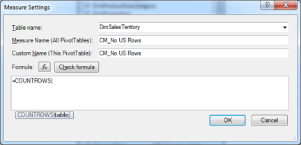
Illustration 45: The Formula, at the Current Point, for Our Second Calculated Measure…
- Type in the letter “F”.
- Via the AutoComplete list that appears, scroll down to the FILTER() function.
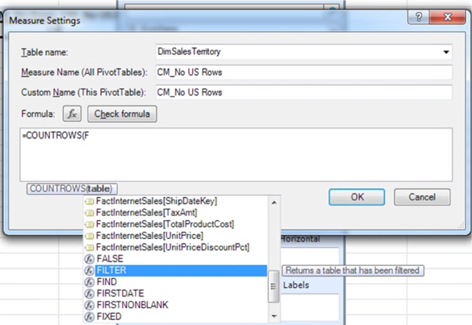
Illustration 46: Scroll to the FILTER() Function within the AutoComplete List
- Click the FILTER() function to select it.
The AutoComplete list is dismissed and the FILTER keyword appears, within the COUNTROWS() function we previously added, in the formula section of the Measure Settings dialog, as presented below.

Illustration 47: The FILTER() Function Appears within the Formula Section of the Dialog
- Because we know that we need now to add the appropriate table name / expression, (we are even reminded of this in the tooltip that appears just under the formula section), begin to type “DimSalesTerritory” to the immediate right of "FILTER(" in the formula section of the Measure Settings dialog.
- As the AutoComplete list again appears, scroll to DimSalesTerritory as depicted below, and click to select it.
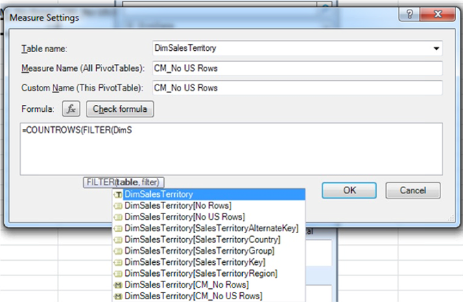
Illustration 48: Select the DimProductSubcategory Table …
- Once the selector is dismissed, and =COUNTROWS(FILTER(DimSalesTerritory appears in the formula section, type in a comma ( “,“ ) to separate the table expression from the filter argument, to be added next.
- Next, begin to type in the DimSalesTerritory table name again, with the intent this time to select the SalesTerritoryCountry column therein.
- Select DimSalesTerritory[SalesTerritoryCountry] in the AutoComplete list.
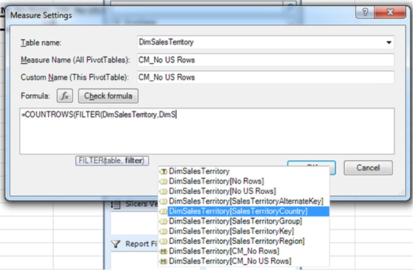
Illustration 49: Select DimSalesTerritory[SalesTerritoryCountry] in the AutoComplete List
- Once the selector is again dismissed, and =COUNTROWS(FILTER(DimSalesTerritory, DimSalesTerritory[SalesTerritoryCountry]
appears in the formula bar, type in an “equals” sign ( “=“ ) to the right of the text appearing in the formula bar.
- Type the following to the immediate right of the “=” sign:
"United States"))
The complete text appears, in the formula section of the Measure Settings dialog, as depicted.
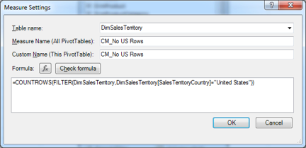
Illustration 50: The Complete Text in the Formula Section of the Measure Settings Dialog
- Click OK key to save the new calculated measure and to dismiss the Measure Settings dialog.
The calculation is saved, and the Measure Settings box is dismissed, once again. The new calculated measure, CM_No US Rows, appears in the PowerPivot Field List, underneath the calculated measure we created earlier, CM_No Rows, and, like that measure, comes preselected, and appears, beneath CM_No Rows, in the Values zone of the PowerPivot Field List, as well as alongside CM_No Rows on the spreadsheet, within the PivotTable, where we now see the numbers “11” and “5.” The PivotTable environment appears, reflecting our addition of the new calculated measure.
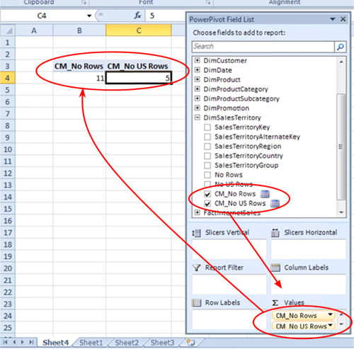
Illustration 51: The PivotTable Environment, Reflecting the Addition of the Second Calculated Measure
Having added two calculated measures at the PivotTable level, we can easily compare the values generated for each with the values generated by its PowerPivot window counterpart. We can therefore see that DAX works in both worlds, in the same manner. Depending upon the use to which we need to put a given calculation, a calculated measure like the above may be better suited than a calculated column. We’ll compare and contrast these two DAX vehicles in the closing section that follows.
Calculated Columns versus Calculated Measures
So how do we determine which is best to use, a calculated column or a calculated measure, in a PivotTable we’re building? When the two approaches generate different “answers,” for reasons of context (more on this to follow), etc., the business requirements will typically drive our choice of options. When either approach will deliver the same desired answer, we will want to select the one that performs more optimally, based upon an understanding of the mechanics behind the calculation involved.
As a consideration in selecting the best approach in the latter case, we should keep in mind that a calculated measure operates upon aggregations that exist “below” the PivotTable (in other words, the aggregations lie “underneath” the DAX evaluation context). The measure works with the aggregations as dictated by the context of the current cell in the PivotTable: the underlying source tables are filtered based upon cell coordinates, and the filter is enforced in accordance with these coordinates. In contrast, when we go the route of a calculated column in the PowerPivot window, it’s important that we grasp the fact that the context of the calculation is the current row; calculated column values are generated via data refreshment, completely independent of user activity at the PivotTable level.
A PowerPivot calculated column is indicated when:
- We wish to see results of the calculation in columns or rows of a PivotTable;
- We wish to place results of the calculation in a vertical or horizontal slicer of a given PivotTable (the calculation has to be available to the slicer of choice, and, thus, has to be an underlying calculated column);
- We need to group / categorize numbers or text (a range of household incomes for customers, a range of values for a sales measure, etc.);
- We want to define an expression that relies solely upon contents of the current row (and not upon calculations occurring within the row).
A PivotTable calculated measure is the appropriate approach to choose when we wish to place results of the calculation in the Values section of the PivotTable – that is, when we want to generate results that are dependent upon user actions / selections within the PivotTable. As an illustration, say we want the calculation to be dependent upon geographical or time / date filters that an information consumer can modify on the fly at the PivotTable level.
As we have noted, some requirements can be met by either calculated columns or calculated measures, although specific definition of the two options might differ, with regard to syntax. In such cases, be sure to test both approaches extensively before reaching a conclusion. One consideration to keep in mind, too, is that, when either approach will deliver the desired result, particularly when dealing with sizeable data volumes, workbook size will be greater when we pick the calculated column option; a calculated measure might therefore prove more optimal from a memory and space consumption perspective.
As a rather obvious consideration, too, keep in mind that any time we select a calculated column from the PowerPivot Field List, we are performing a SUM upon that column. As an example, if we return to our example in the practice section above, and place a check in the checkbox to the immediate left of the No US Rows calculated column within the expanded DimSalesTerritory table, the calculation is summed (we can see the calculation itself by right-clicking the new entry in the Values zone, and examining the formula bar at the bottom of the Measure Settings dialog that appears) as shown.
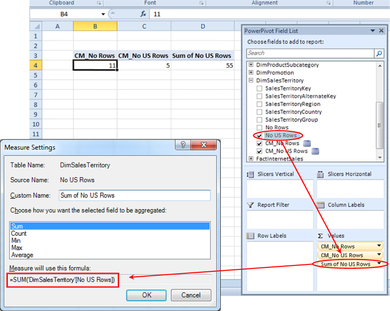
Illustration 52: Summing of the Calculated Column When Selected as Value in PivotTable
One rather obvious consequence of the summing we see here can be a “double operations” effect. We can easily see in this example that the Sum of Non US Rows is 55, as opposed to the value of 5 that is returned at the PowerPivot level, where the calculated column returns a 5 on each of the 11 rows in the table, or the value of 5 that is returned via the CM_Non US Rows calculated measure at the PivotTable level. The “double operation” of the calculation occurs when the calculated column value of 5 is summed for all 11 rows: in effect, “summing a sum” occurs. The point here is simply to illustrate the importance of realizing “what we are asking for” when we choose a calculated column as a value, and ascertaining that the returned value is, indeed, what we expect it to be.
- From the main menu of the workbook, select File -- Save As …
- Name the file ST_DAX02-1.xlsx, and save it in a meaningful location.
- Exit Excel 2010 as desired.
When working with PowerPivot, understanding the nature and operation of, the differences between, and the optimal uses for, calculated columns and calculated measures is critical to sound and efficient reporting and analysis with this powerful tool. We will work with these concepts throughout the Levels of Stairway to PowerPivot and DAX, embellishing and enhancing our technique as the series evolves. Practice and further experimentation with these and other components will ensure that we become fluent in the many options and opportunities that PowerPivot offers the knowledgeable user.
Summary
In this Level of the Stairway to PowerPivot and DAX series, we exposed the DAX COUNTROWS() and FILTER() functions. We discussed the general purposes and operation of the functions, and then focused upon ways in which each of these functions can be employed, first in standalone examples for COUNTROWS(), and then in situations where we employed COUNTROWS() and FILTER() together, to achieve results similar to those we might need to generate for clients or employers in our own environments. As part of our discussion, we examined the syntax surrounding each function, undertaking illustrative examples of the uses of the each in practice exercises, and the briefly discussed the results datasets we obtained in the practice examples.
In addition to introducing the COUNTROWS() and FILTER() functions, we examined ways to access the PowerPivot calculated columns we had constructed from a PivotTable we built in the section that followed. We then created calculated measures, again employing the COUNTROWS() and FILTER() functions, to replicate the calculated columns we had created earlier in the PowerPivot window. We compared and contrasted calculated columns and calculated measures in general, discussing criteria to consider in choosing which of these two calculation approaches to take in meeting business requirements in our own environments.
