Introduction

In earlier articles we worked with decision trees, clusters, Naive Bayes, and Neural Network Algorithms. The examples used were related to predicting the probability of a customer buying a bike. All the algorithms used the same input and the output was a % of the probability.

You can read the previous articles in this series using the links below:

• An introduction to data mining
• Decision trees
• Clusters
• Naïve Bayes
• Neural Network

The Time Series Algorithm will be a little different, and it is a separate sample with different inputs and outputs. We will, however, use the Adventureworks samples for this demo. The linear regression algorithm is used to predict the linear behavior between an independient variable and a dependent one.

A good example of a typical use of this algorithm is the house price. Let's say that the price of a house in June is $100,000, in July it is $100,100, in August it is $100,250, and in September, it's $100,300. If we want to predict the price of the house in October, November and December, we can predict the price behavior using a time series:

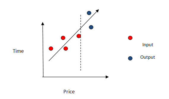
The image above ilustrates how the time series works. The input is used to predict the future. The red dots are the input and the blue ones are future values predicted.

If we have the historical prices of houses, cars, or any product, we can predict future prices in the future.

Requirements

For this example, I am using the Adventureworks Multidimensional project and the AdventureworksDW Database. You can download the project and the database here: http://msftdbprodsamples.codeplex.com/releases/view/55330

Getting started

In order to start we are going to work with the [dbo].[vTimeSeries] from the AdventureworksDW database:

SELECT  [ModelRegion]
      ,[TimeIndex]
      ,[Quantity]
      ,[Amount]
      ,[CalendarYear]
      ,[Month]
      ,[ReportingDate]
  FROM [AdventureWorksDW2012].[dbo].[vTimeSeries]
  order by TimeIndex

You can see the results here:

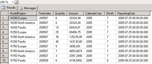
As you can see, the table shows the TimeIndex, which includes the Year and the Month. The ModelRegion contains the model per region, the quantity and the Amount contains data about the sales in a specific date for the model. CalendarYear and month contain the Year and the Month and the product.

If you run the queries to find the maximum and minimum for the dates, you will notice that this view contains sales from the Year 2005 to the year 2008.

Select max(TimeIndex)
 FROM [AdventureWorksDW2012].[dbo].[vTimeSeries]

Result:  200806

The max value is June, 2008

Select min(TimeIndex)
 FROM [AdventureWorksDW2012].[dbo].[vTimeSeries]

Result:  200507

The min value is July, 2005.

The times series algorithm will predict future sales (the quantity and the amount of future months). There is already an example in the Adventureworks download created. The Data Mining Structure name is Forecasting,which you can see below:

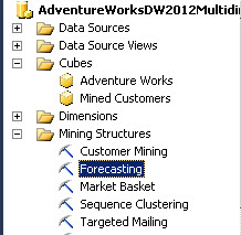
If you double click the Forecasting structure, you will find the information displayed:

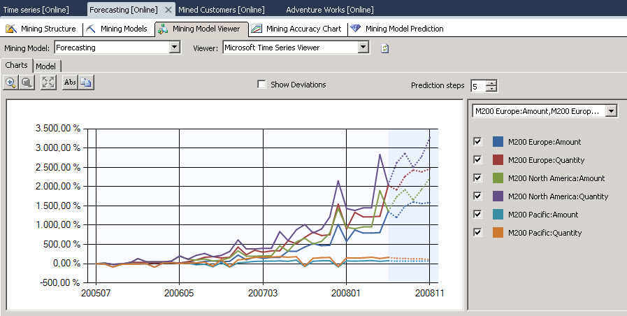
The data mining using Time Series shows a straight line for the input data and a dotted line for the predicted data.

We are going to create a similar example using the [dbo].[vTimeSeries] view.

Steps

1. In the AdventureWorks project right click in the mining structures and select the option New Mining Structure.

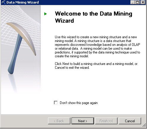
2. In the Welcome Wizard, press next

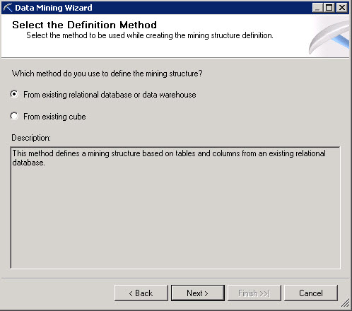
3. In the select the definition, method choose the from existing relational database option.

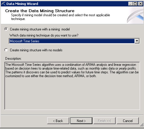
4. This part is new, select the Microsoft Time Series mining technique.

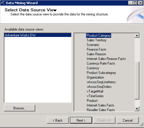
5. In the available Data Source select the only one available (Adventure Works DW).

6. In the specify table, select the vTimeSeries View. This is the view than we mentioned in the getting started section with the input information.

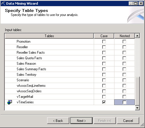
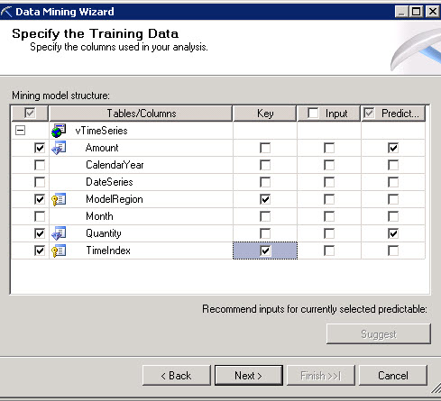
7. The keys used are the modelRegion and the timeIndex. These attributes contains the Bike models and the Data of the sales. We are going to predict the Amount and Quantity.

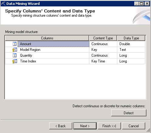
8. The next option is used to specify the data types. Leave the default values.

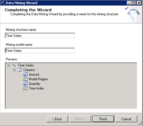
9. In the Completing the wizard windows specify a structure and model name:

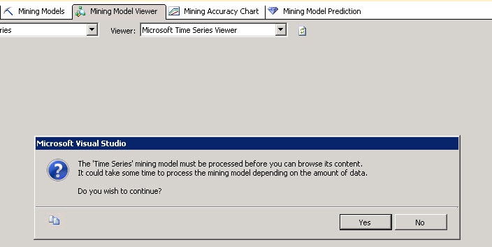
10. In order to see the results, go to the mining model viewer tab. You will receive a message to process the model. Press Yes to the yes/no question windows.

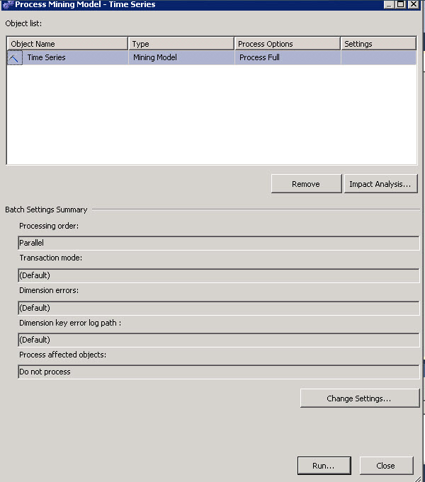
11. In the process mining model press Run.

12. You will receive a Final window to accept the process and then you will see the following result:

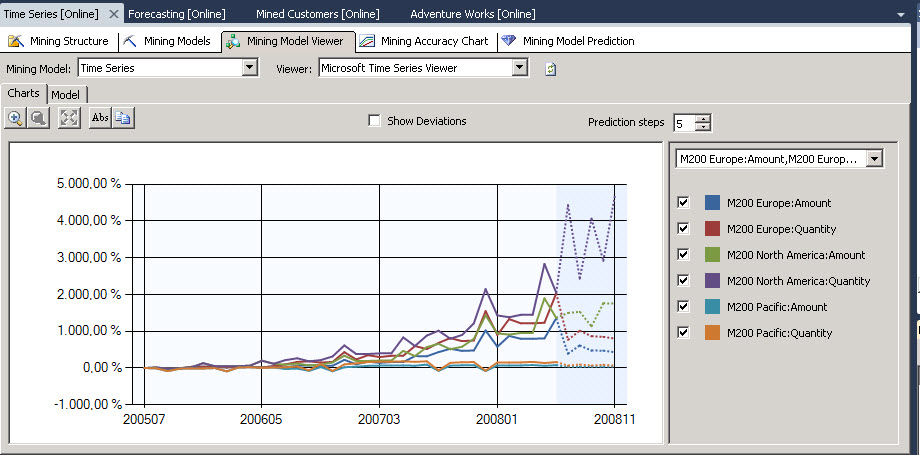
13. As you can see, you have the input values from 2005 until the middle of 2008 after that you can notice pointed lines which are the predictions for the future.
14. In order to have a specific values for specific models. We will use mining model prediction.
15. In the mining model prediction tab select a Model.

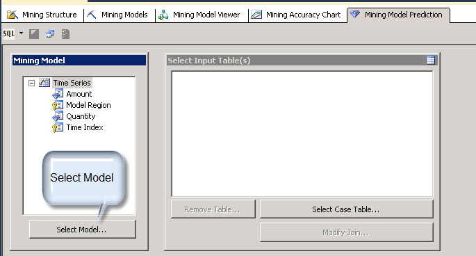
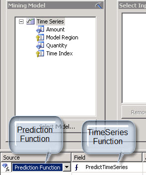
16. In the source section in the combobox select prediction function and in the field select timeSeries Function. We are using the function time Series to predict the future.

17. Drag and drop the amount in the criteria field and add a coma 4 after the amount. 4 is the number of values displayed and predicted for the Amount.

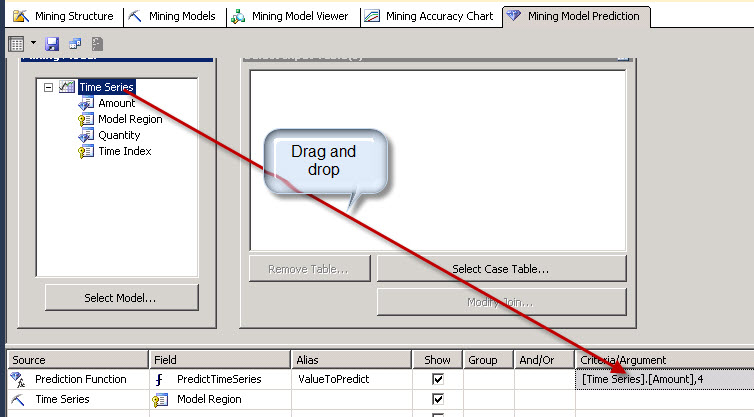
18. Now, we are going to add the model. In order to do that in the source field, add the Time Series in the source field and model region in the field.

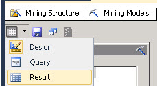
19. Let’s watch the results:

20. We can now observe the values per model. In the following example we will match the amont sold by the M200 Europe model.

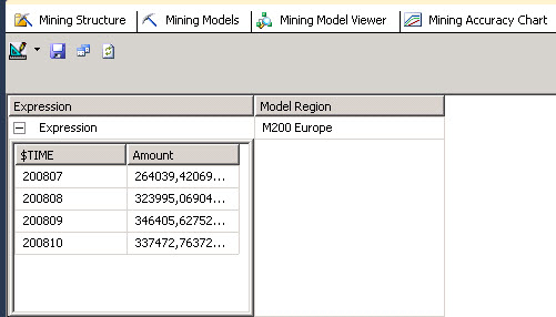
As you can see, you can now predict sales and values using the time series algorithm.

Conclusion

In this tutorial, we learned how to use the Time Series Data Mining algorithm to predict values over the time. This is a simple algorithm, but it is different than other algorithms used in earlier chapters. This algorithm requires less input data and can predict multiple values over time.

In the next chapters we will talk about other data mining algorithms.

References

http://msdn.microsoft.com/en-us/library/fb22cffa-ac99-4d34-ac4a-9c93068e33e8