This is the fourth article about data mining. If you want to find the other parts they are:
- Data Mining Introduction part 1 - Getting started with the basics
- Data Mining Introduction part 2 - Decision Trees
- Data Mining Introduction part 3 - The Cluster Algorithm
In the last chapter we already created a Data Mining Model using the cluster algorithm. In this new article I will introduce a new algorithm: the Naïve Bayes Algorithm.
The Microsoft Naïve Bayes Algorithm
The Microsoft Naïve Bayes is based in the Bayes theorem. This theorem was formulated by Thomas Bayes an English Presbyterian minister (and a mathematician).

In fact the Bayes’ theorem was presented to the Royal Society after Thomas dead (at least he is famous now and we are talking about him in the most visited SQL Server site in the world!).
Microsoft created an algorithm based on this theorem. We call this algorithm Naïve because we do not consider dependencies in this algorithm. I am not going to show you Bayesian formulas because Microsoft has an easy to use interface that does not require knowledge of the mathematical algorithm. That part is transparent to the user.

In few words what the algorithm does is to show the probability of each attribute to do a certain thing.
In the Adventureworks example used in the tutorial we have a list of prospective customers to buy a bike. With the algorithm we show the percentage of people who will buy a bike according to isolated characteristics.
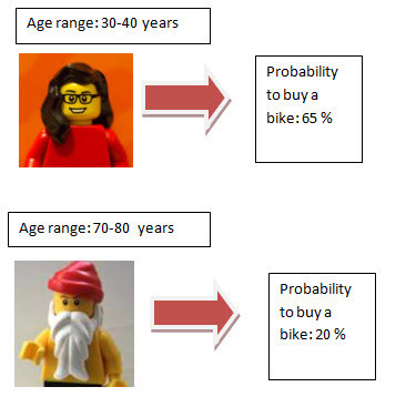
The algorithm classifies the customers per age and it shows the same probability to buy a bike according to the age range. It will do the same process per each attribute. It is naïve because it does not consider the dependencies between attributes.
As you may notice with the information just provided, it is a simple algorithm (that’s why we call it naïve) and it requires fewer resources to compute the information. This is a great algorithm to quickly start researching relationships between attributes and the results.
For example the address attribute can or cannot be an attribute that affects the probability to buy a bike. In fact, there is a direct relationship between the address and the probability to buy a bike because some neighbors usually can use the bike there and some cannot because of the traffic. Unfortunately, it is really hard to group all the addresses so it is a good question if we need to include the attribute in the model.
If you are not sure which attributes are relevant, you could test the attribute using this algorithm.
Requirements
We are still using the Adventureworks databases and projects from the Data Mining Part 3.
In that chapter we already created a model to predict the probability of a customer to buy bikes using decision trees and clusters. The algorithm already used a view as an input and we created the input to feed the algorithm. We will use the same information to create the Naïve Bayes Algorithm.
Getting started
- We are going to open the AdventureWorks Project used in earlier versions and open it with the SQL Server Data Tools (SSDT).
- In the solution Explorer, we are going to move to the Mining Structures.
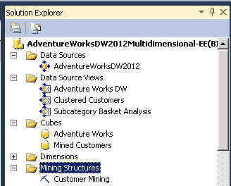
- In the Mining Structures folder double click in Targeted Mailing. It is the sample to verify which customers are prospective buyers to email them.

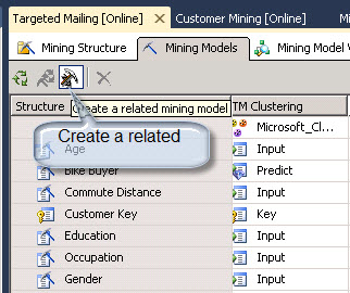
- Click in the Mining Model Tab and Click the icon to create a mining model.
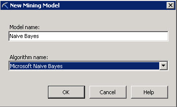
- In the New Mining Model Window select the name of the model. You can specify any name. Also select the Naïve Bayes Algorithm.
- This is very important. The Naïve Bayes does not support continuous data. In this sample, it does not support the Yearly Income. That is why you will receive the following Message:

8. Discrete data means that the number of values is finite (for example the gender can be male and female). Continues is a number of values that is infinite (for example the number of starts, grains, the weight, size). The Naïve Bayes supports only discrete data.
9. It cannot work with data like the salary, taxes that you pay extra incomes and other type of data that is continuous. The algorithm classifies in groups the attributes according to values. If it has infinite number of values it cannot classify the attributes. That is why it excludes this type of attributes.
In the Mining Structure tab, you can optionally ignore some inputs in the model. By default the Yearly Income is already ignored if you press Yes to the question to ignore the column.

9. Now click in the Mining Model Viewer Tab and select the Naïve Bayes just created.

10. You will receive a message to process the new model. This new model will be loaded with the data when you process it. Click yes in the message.

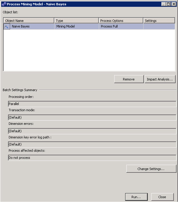
11. In the Process Mining Model you need to press the run button. This button will start processing the information from the views and get results using the algorithm.
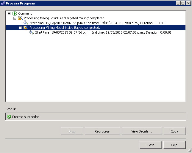
12. At the end of the process you will receive a message with the start day, duration of the process.
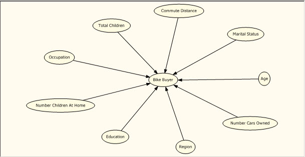
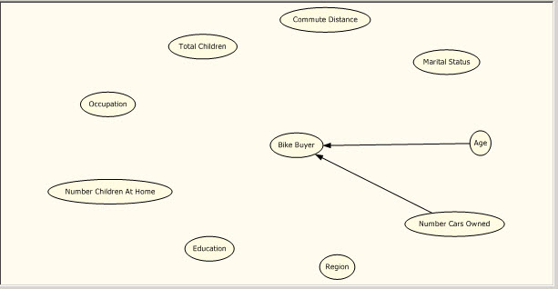
13. The first tab is the Dependency network. This is similar to the decision tree. You will find which the main factors to buy a bike are. At the beginning you will see that all the attributes have an influence in a customer to buy a bike.
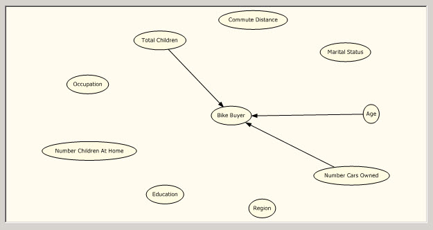
14. However, if you move the dependency bar, you will find that the main factor to buy a bike is the Number of cars. That means that depending of the cars you own, the probabilities to buy a bike changes a lot.
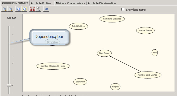
15. The second factor is the age. It means that the age is the second factor to buy a bike or not.
16. The third factor is the number of children. Maybe if you have many children you will want to buy more bikes (or maybe none because it is too dangerous).
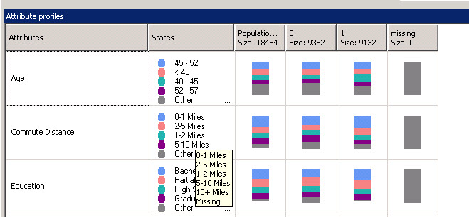
17. The other tab is the Attribute profiles tab. This is nice graphical information that helps you classify the attributes information. For example, most of the people that buy bikes are 45-52 years old. Also the commute distance is from 0 to 1 mile. You can analyze the whole population, the people who buy bikes (1 Size) and the people who do not buy (0 size).
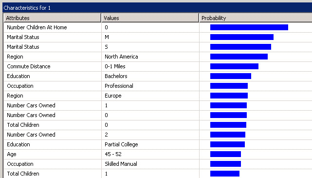
18. There is another tab named attribute characteristics. You can see the probability to buy a bike according to specific attributes. For example the people will buy a bike if they do not have children at home and they are males and single.
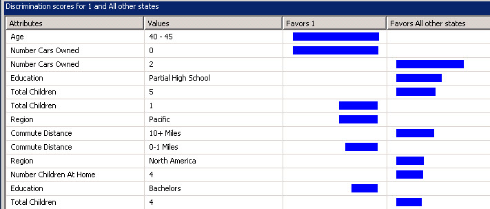
19. The discrimination score tab, show you the attributes and the main reasons related to attributes to buy or not to buy a car.
For example the people without a car may want to buy a bike, but people with 2 cars will not like to buy a bike. People with 5 children won’t buy a bike (because controlling 5 kids in the street will drive them crazy) while people with 1 child will like to buy a bike.
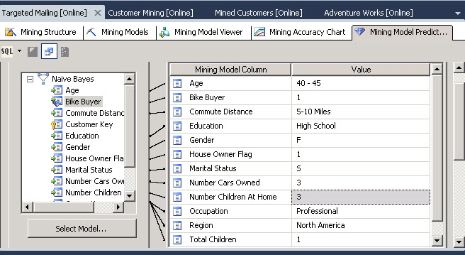
20. Finally we will ask to our model what if the probability to buy a bike of a prospective customer who is 40-45 years old, with a commute distance of 5-10 miles, with high school, female, single, house owner, with 3 cars and 3 children to buy a bike. For this purpose we will go to the mining model prediction tab.
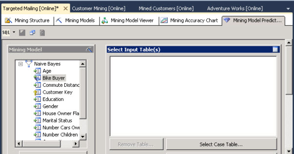
21. Make sure in the Mining Model that the Naïve Bayes model is selected and press the select case table button.
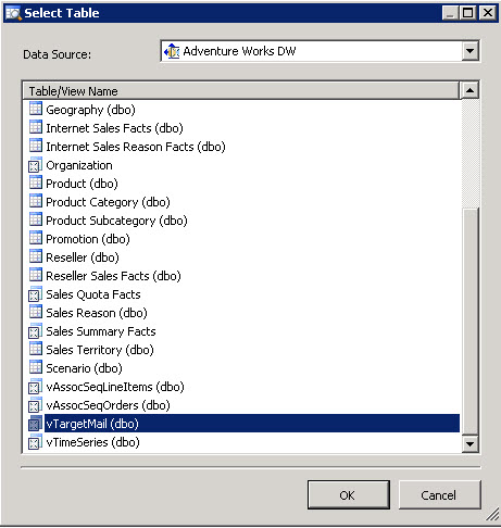
22. In the select table Window, you select the table that you will use to feed you Naïve Bayes algorithm. In this case, the dbo.TargetMail contains a list of prospective customers to send them mails.
23. In the select Input Table, select the option singleton. This option let’s you create a single query of a single user with specific characteristics.
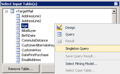
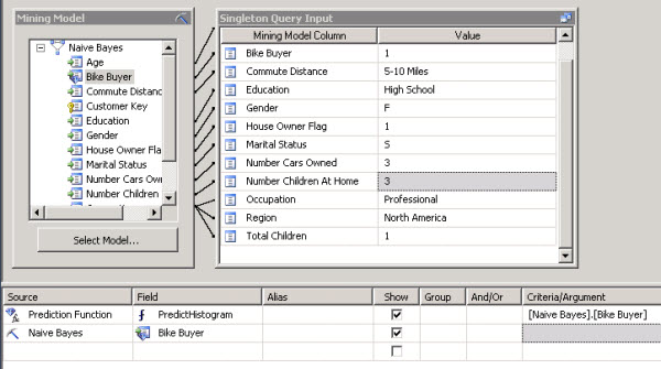
24. Now write the characteristics specified in step 20 with the characteristics of the user (age, number of children, education and so on).
25. Also add the prediction function named PredictHistogram. This function provides you a histogram with the probability to buy a bike. Add the Naïve Bayes criteria and the Naïve Bayes source.
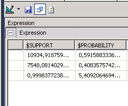
26. Finally, go to the results.

You will see that the probability to buy a bike for the customer with the information provided is 0.5915 (59 %).
Conclusion
In this chapter we used a new algorithm or method named Microsoft Naïve Bayes. We learned that it is a simple algorithm that does not accept continues values in the attributes. It only accepts discrete values. This algorithm is used to get fast results and to analyze individual attributes specially. In a next chapter we will explain more Data Mining algorithms.
The way to predict data is similar no matter the algorithm used.

