Cardinality

This is a term originally from Mathematics, generally defined as “The number of objects in a given set or grouping”. In SQL we’re continually dealing with sets so this becomes a very relevant topic, which in our context is just the “number of rows”.

When you have a query across multiple tables there any many ways in which SQL Server could decide to physically go about getting you the results you want. It could query and join the tables in any order and it could use different methods for matching records from the various tables you have joined together. It also needs to know how much memory to allocate for the operation – and to do that it needs to have an idea of the amount of data generated at each stage of processing.

A lot of this requires cardinality estimation, and SQL Server uses something called Statistics objects to perform that calculation.

Let’s look at a simple example:

SELECT *

FROM Person.Person p

INNER JOIN Person.[Address] a

ON p.AddressId = a.AddressId

WHERE p.LastName = 'Smith'

AND a.City = 'Bristol'

When it comes to gathering the results for this query there are a number of ways the database engine could go about it. For instance:

a) It could find all the records in the Person table with a LastName of Smith, look each of their addresses up and return only the ones who live in Bristol.

b) It could find all the Addresses in Bristol, look up the people associated with each address and return only the ones called Smith.

c) It could grab the set of people called Smith from the People table, grab all the addresses in Bristol, and only finally match up the records between those two sets.

Which of those operations is going to be most efficient depends very much on the number of records returned from each table. Let’s say that we have a million people called Smith, but there’s only one address in our whole database that is in Bristol (and let’s say that address does actually belong to someone called Smith).

In the first method above I would grab the million Smiths and then look their address up one by one in the address table until I found the one that lived in Bristol.

If I used method b) though, I would find the one matching address first, and then I would simply look up the owner of that address. Clearly in this rather contrived example, that’s going to be a lot quicker. So if SQL knows ahead of time roughly how many records to expect from each part of the query, hopefully it can make a good decision about how to get the data.

But how can it work out how many rows will be returned without actually running the query?

Statistics

That’s where statistics objects come in. SQL Server maintains in the background data that equates to a histogram showing the distribution of the data in certain columns within a table. It does this any time you create an index – statistics will be generated on the columns the index is defined against, but it also does it any time it determines that it would be useful. So if SQL encounters a Where clause on Person.LastName – and that column isn’t involved in a useful index, SQL is likely to generate a statistics object to tell it about the distribution of data in that column.

I say “likely to” because it actually depends on the settings of your SQL instance. Server configuration is beyond the scope of this post but suffice to say you can let SQL automatically create Statistics objects – or not. You can let it automatically update them when the data has changed by more than a given threshold – or not. And you can specify whether updates to statistics should happen asynchronously or synchronously – i.e. in the latter case if your query determines that statistics needs updating then it will kick that off and wait until the update is complete before processing the query.

It’s generally recommended that auto creation and updating is on, and async updating is off.

Viewing Statistics Objects

Let’s have a look at some actual statistics and see what they hold. There are a couple of ways of doing this, the first is through SSMS. If you look under a table in the object browser you will see a Statistics folder which holds any statistics objects relating to that table:

In the above example you can see some that have friendly names, these are Statistics that  are related to an actual index that has been defined on the table and they have the same name as the Index – e.g. IX_Address_StateProvinceId.

You’ll also see we have some prefixed _WA_Sys and then with some random numbers following. These are statistics objects that SQL has created automatically on columns that aren’t indexed – or at least they weren’t indexed at the time the Statistics objects were created.

You can open these up with a double-click and see what’s inside:

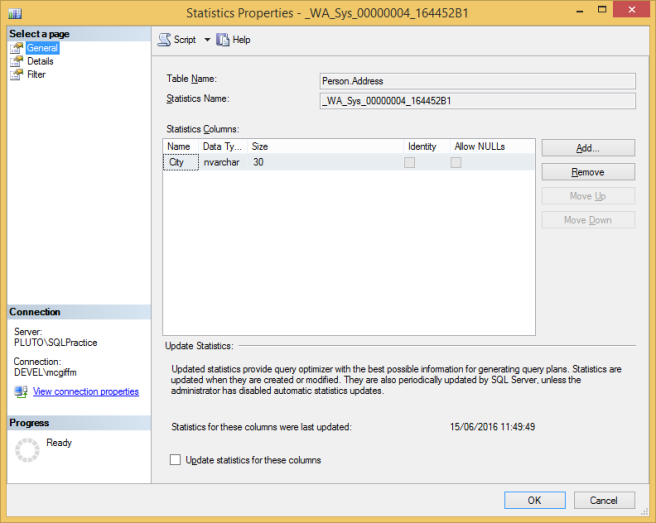
This is the General tab you open up to. You’ll see it tells you what table the Statistics are for and what column(s). There are options for adding columns and changing the order – but you never really need to do this – as well as information to tell you when the statistics were last updated, and a check box if you want to update them now.

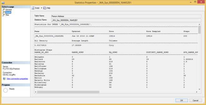
In the details tab there’s a lot more info:

I don’t find this the easiest display format to work with though, so rather than delving into what everything means here let’s look at the other way you can view statistics, which is by running the following command:

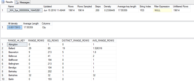
DBCC SHOW_STATISTICS('Person.Address', '_WA_Sys_00000004_164452B1')

The format is straightforward, you just specify the table you are interested in the Statistics for, and the actual name of the Statistics object you want. You can see the same information as if you double-clicked on it, but the results are output in the results pane like any other query and are (I think) a lot easier to read. Allegedly there will soon be a third way in SQL Server to view Statistics as DBCC commands are considered a bit “clunky” – but we don’t know what that will look like yet.

The command outputs three resultsets:

This post is just an introduction to statistics – and generally you don’t need to know that much, it’s just handy to understand the basics. So let’s just run over the key bits of information you can see above:

First of all in the first recordset – otherwise know as the…

Stats Header

Rows – is the number of rows in your table

Rows Sampled – this is how many rows were sampled to generate the statistics. SQL can generate or update statsitics using sampling rather than reading all the rows. In this case you’ll see it did actually read the whole table.

Steps – If you imagine the statistics as a bar chart – this is the number of bars on the chart. Statistics objects have a maximum of 200 steps so if you have more distinct values in your column than that they will be grouped into steps.

Density – This is supposed to be the probability of a row having a particular value (calculated as 1 / Number of Distinct values in column). According to books online “This Density value is not used by the query optimizer and is displayed for backward compatibility with versions before SQL Server 2008.”  I am using SQL 2012, and this number is just plain incorrect so don’t use it…

Recordset Number 2: The Density Vector

All Density – this is the accurate version of the Density statistic described above. So your probability of a given row having a specific value is about 0.0017. That’s a little less than one in 500. I happen to know there are 575 different Cities in the table so that makes sense. Sometimes SQL will use this value to form a plan – if it knows you’re going to search this table for a specific City and it doesn’t know that City when it makes the plan, then it could guess that about 1/500th of the rows will match your criteria.

Average Length – Is what it says on the can. The average length of data in this column.

Columns – The names of any column measured in this statistics objects. You can have statistics across multiple columns but I’m not going to cover that in this post. In this case it tells us these statistics are based on the “City” column.

Recordset Number 3: The Histogram

This last recordset shows the distribution of the data, and is what you could effectively use to to draw a graph of the relative frequencies of different groups of values. Each row represents a step – or bar on the bar chart – and as mentioned above there can be a maximum of 200 steps. So you can see, a statistics object is quite lightweight, even for a massive table.

RANGE_HI_KEY – This upper limit of each step, so each step contains all the values bigger than the RANGE_HI_KEY of the last step, right up to and including this value.

RANGE_ROWS – This is how many rows in the table fall in this range – not including the number that match the RANGE_HI_KEY itself.

EQ_ROWS – The number of rows equal to the HI_KEY

DISTINCT_RANGE_ROWS – The number of different values in the range that there is data for (excluding the HI_KEY).

AVERAGE_RANGE_ROWS – The average number of rows for a given value within the range.

That’s a whistle-stop tour of the Statistics SQL Server holds on your data.

The algorithms that SQL then uses to calculate the number of rows for a given part of your query are pretty transparent when there’s just one column involved. If we look at the above example and let’s say you wanted to look up the rows where the City is “Abingdon” – the statistics tell us there is 1 matching row and that’s the figure SQL will use for cardinality estimation. Where a value is within a range then it will use a calculation based on the AVERAGE_RANGE_ROWS.

When there’s multiple columns involved it’s more complicated there are various algorithms and assumptions that come into play. If you’re interested in digging deeper, one very good resource is the Whitepaper on the 2014 Cardinality Estimator written by Joe Sack: https://www.sqlskills.com/blogs/joe/optimizing-your-query-plans-with-the-sql-server-2014-cardinality-estimator/

Conclusions

The main takeaway from this should just be the understand the extent – and limitations – of the information about the distribution of your data that SQL holds in the background.

If, when you’re tuning queries, you notice that the estimated row counts don’t match the actual, then this could be encouraging SQL to form a bad plan for the query. In these cases you might want to investigate what’s going on with the statistics.

Maybe your query is written in a way that it can’t use statistics effectively, one example of this can be where you store constant values in variables, then query using that variable in a WHERE clause. SQL will then optimise based on the average, rather than on your actual value.

Maybe the plan is based on one data value that has a very different cardinality to the one currently being queried. For instance when you first run a stored procedure, the plan is formed based on the parameters passed. Those parameters could have a cardinality that is quite different to those used in later executions.

Maybe the statistics are out of date and need refreshing. Stats get updated when approximately 20% of the data in the table changes, for a large table this can be a big threshold, so current statistics may not always hold good information about the data you are querying for.

Or maybe SQL is doing as good a job as it can with the information it has at its disposal. You might need to work out how you can give it a little extra help.

This is in only intended to be an introduction to Statistics objects. If you want to find out more, your favourite search engine is your friend. For the moment, I hope this makes it clear what Statistics objects are, what they are used for, and why they are important.