By Steve Bolton

…………In the last installment of this series of amateur self-tutorials on using SQL Server to identify probability distributions, we saw how devices like probability plots can provide simple visual confirmation of a dataset’s shape. I considered doing a quick detour into Q-Q plots, but decided against it because of their simplicity; instead of putting values for the distribution being tested on the horizontal axis, Q-Q plots chop them up into partitions of equal size, a task that is obviously trivial to implement with NTILE. I’m more eager to discuss skewness and kurtosis, two of the oldest, tried-and-true measures of goodness-of-fit[1] – particularly for the normal or “Gaussian” distribution, i.e. the bell curve – precisely because they are often easy to spot with the naked eye. They are numerical measures rather than visualizations, but are often self-evident within graphics like histograms. For example, the third histogram in my recent post Outlier Detection with SQL Server Part 6.1 – Visual Outlier Detection with Reporting Services is a striking examples of a highly skewed column, while the one below it obviously follows a bell curve more closely and has relatively low skewness and kurtosis; later in this article, I’ll run some sample T-SQL code against the same data to derive hard numbers for both. I’ve seen several good explanations of the meanings of skewness and kurtosis in sources at various sites on the Internet, including one of my favorites, the National Institute for Standards and Technology’s Engineering Statistics Handbook, which defines them thus: “Skewness is a measure of symmetry, or more precisely, the lack of symmetry. A distribution, or data set, is symmetric if it looks the same to the left and right of the center point…Kurtosis is a measure of whether the data are peaked or flat relative to a normal distribution. That is, data sets with high kurtosis tend to have a distinct peak near the mean, decline rather rapidly, and have heavy tails. Data sets with low kurtosis tend to have a flat top near the mean rather than a sharp peak. A uniform distribution would be the extreme case.”[2] Another succinct explanation is given by Tompkins County Community College adjunct faculty member Stan Brown, who says that “The histogram can give you a general idea of the shape, but two numerical measures of shape give a more precise evaluation: skewness tells you the amount and direction of skew (departure from horizontal symmetry), and kurtosis tells you how tall and sharp the central peak is, relative to a standard bell curve.” [3]
…………I already had some experience with both measures way back in A Rickety Stairway to SQL Server Data Mining, Part 14.2: Writing a Bare Bones Plugin Algorithm and A Rickety Stairway to SQL Server Data Mining, Part 14.6: Custom Mining Functions, when I made crude attempts to implement skewness and kurtosis in SSDM in order to illustrate the capabilities of its custom algorithms and functions. That called for fairly simple stats which wouldn’t distract from the main mission; I didn’t really even make much of an effort to understand them, because it wasn’t germane to the lesson at hand. Since then I’ve discovered that it’s easier for me to grasp both stats by viewing them as numerical measures of lopsidedness on a histogram that is divided into imaginary stripes, in which skewness detects how uneven a distribution is from one vertical band to another, whereas kurtosis measures how squashed the distribution curve is on the horizontal axis. Either way you look at it, the measures are still simple enough to explain in layman’s terms, which is one of the strengths of the set of normality tests built from them.
…………The most well-known extension of these somewhat forgotten stats is the Jarque-Bera Test, which only dates back to the 1970s despite being one of earliest examples of normality testing. All of these measures have fallen out of favor with statisticians to some extent, for reasons that will be apparent shortly, but one of the side effects of this is that it is a little more difficult to find variations on them that are more suited to the unique needs of the SQL Server community. One of the strengths of data mining on database servers like SQL Server is that you typically have such an enormous number of records to draw from that you can actually perform calculations on the full population, or a proportion close to it. In ordinary statistics, however, you’re often limited to making inferences based on small samples of just a few dozen or a few hundred rows, out of a much larger population that is often of unknown size; the results can still be logically valid, but often only if other preconditions are met on the data (including normality tests, which are often not performed). For that reason, I usually prefer to leverage SQL Server’s fast set-based retrieval methods to quickly calculate statistics on full populations whenever possible, especially when there are simpler versions of the mathematical formulas available for the full dataset. Skewness and kurtosis are among those measures that can be computed in a simpler way when using the whole population[4], but I’ve opted here to use the more intensive formulas for sample skewness and sample kurtosis for one reason only: it might be possible to substitute population skewness and kurtosis for their sampling counterparts in the formulas for the Jarque-Bera Test, but I can’t find any online sources that mention such a swap. I suspect that it probably would be logically valid, but I took the more conservative approach in Figure 1 by employing the usual Jarque-Bera formula, which really isn’t much more difficult to compute.[5]

Figure 1: Code for the Jarque-Bera Test Procedure
ALTER PROCEDURE [Calculations].[NormalityTestJarqueBeraSkewnessAndKurtosisSP]
@DatabaseName as nvarchar(128) = NULL, @SchemaName as nvarchar(128), @TableName as nvarchar(128),@ColumnName AS nvarchar(128), @PrimaryKeyName as nvarchar(400)
AS

DECLARE @SchemaAndTableName nvarchar(400),@SQLString nvarchar(max)
SET @SchemaAndTableName = @DatabaseName + ‘.’ + @SchemaName + ‘.’ + @TableName
SET @SQLString = ‘DECLARE
@Mean float,
@StDev float,
@Count as bigint,
@One float = 1,
@RecpiprocalOfNSampleSize float,
@DifferenceFromSampleMeanSquared float,
@DifferenceFromSampleMeanCubed float,
@DifferenceFromSampleMeanFourthPower float,
@SampleSkewness float,
@SampleKurtosis float,
@JarqueBeraTest float 

SELECT @Count = Count(‘ + @ColumnName + ‘), @Mean = Avg(CAST(‘ + @ColumnName + ‘ AS float)), @StDev = StDev(‘ + @ColumnName + ‘)
FROM ‘ + @SchemaAndTableName + ‘
WHERE ‘ + @ColumnName + ‘ IS NOT NULL

SELECT  @RecpiprocalOfNSampleSize = @One / @Count

SELECT  @DifferenceFromSampleMeanSquared = SUM(Power(DifferenceFromSampleMean, 2)) OVER (ORDER BY ‘ + @PrimaryKeyName + ‘ ASC),
       @DifferenceFromSampleMeanCubed  = SUM(Power(DifferenceFromSampleMean, 3)) OVER (ORDER BY ‘ + @PrimaryKeyName + ‘ ASC),
       @DifferenceFromSampleMeanFourthPower  =SUM(Power(DifferenceFromSampleMean, 4)) OVER (ORDER BY ‘ + @PrimaryKeyName + ‘ ASC)
FROM (SELECT ‘ + @PrimaryKeyName + ‘, CAST(‘ + @ColumnName + ‘ AS float) – @Mean as DifferenceFromSampleMean — make a single pass across the table?
              FROM ‘ + @SchemaAndTableName + ‘
              WHERE ‘ + @ColumnName + ‘ IS NOT NULL) AS T1

SELECT @SampleSkewness = (@RecpiprocalOfNSampleSize * @DifferenceFromSampleMeanCubed)  /(Power((@RecpiprocalOfNSampleSize * @DifferenceFromSampleMeanSquared), 1.5))

SELECT @SampleKurtosis = (@RecpiprocalOfNSampleSize * @DifferenceFromSampleMeanFourthPower)  /(Power((@RecpiprocalOfNSampleSize * @DifferenceFromSampleMeanSquared), 2))

SELECT @JarqueBeraTest = CAST((CAST(@Count AS float) / CAST(6 AS float)) AS Decimal(38,12)) * CAST((Power(@SampleSkewness, 2) + (0.25 * Power((@SampleKurtosis -3), 2))) AS Decimal(38,12)) 

SELECT @JarqueBeraTest AS JarqueBeraTest, @SampleSkewness AS SampleSkewness, @SampleKurtosis AS SampleKurtosis, @SampleKurtosis – 3 AS ExcessKurtosis, @Mean AS  Mean, @StDev AS StDev
— to debug the internal calculations, uncomment the rest of this line, @DifferenceFromSampleMeanSquared, @RecpiprocalOfNSampleSize, @DifferenceFromSampleMeanSquared, @DifferenceFromSampleMeanCubed, @DifferenceFromSampleMeanFourthPower
‘

–SELECT @SQLString — uncomment this to debug dynamic SQL errors
EXEC (@SQLString)

…………The end of the final SELECT can be uncommented to debug the internal calculations. I’ve also reserved the second-to-last line for a SELECT that can be uncommented to debug the dynamic SQL string, as is standard in most of my procedures. Much of the initial code ought to be familiar to reader of this series and the one on outliers, since I use many of the same parameters and internal variables, and apply some of the usual preliminary SET operations on them. As usual, I calculate the values of some reusable internal stats and then cache them in dynamic SQL variables so that we don’t have to recalculate them again, as in the case of the reciprocal of the count and the deviation computation in the lowest-level subquery. I’m experimenting with declaring constants like 1 to high precision data types to prevent situations where SQL Server sometimes truncates the values during calculations, which can lead to erroneous results or at best, messy code full of casts deep within subqueries to avoid such errors. One departure from the norm is the use of floats rather than the decimal data type in the dynamic SQL calculations. The square, cube and quartic operations can result in really high and low values, which may in turn cause divide by zero errors if they’re rounded down to nothing or arithmetic overflows if they’re rounded too high, so I resorted to using float data types for the first time in any of my mistutorial series. This may entail some loss of precision in the internal calculations, but shouldn’t have much an effect on the final test statistic. It is not uncommon for this result to seem outlandishly high when the underlying distribution is abnormal.[6]

Figure 2: Sample Results from the Duchennes Table and HiggsBosonTable
EXEC   [Calculations].[NormalityTestJarqueBeraSkewnessAndKurtosisSP]
              @DatabaseName = N’DataMiningProjects’,
              @SchemaName = N’Health’,
              @TableName = N’DuchennesTable’,
              @ColumnName = N’LactateDehydrogenase’,
              @PrimaryKeyName = N’ID’

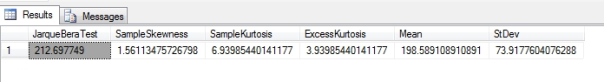
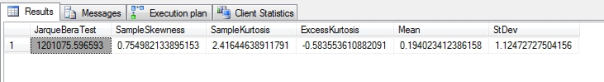
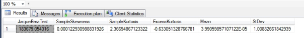
…………The query in Figure 2 produced the results in the graphic immediately below it, in which I tested the procedure on the LactateDehydrogenase column of a dataset on the Duchennes form of muscular dystrophy, which is made publicly available by Vanderbilt University’s Department of Biostatistics. The procedure performed surprisingly well when deriving the other two result sets, clocking in at 3:43 and 3:42 minutes on the first two float columns of the Higgs Boson Dataset, which I downloaded from the University of California at Irvine’s Machine Learning Repository and converted into a SQL Server table. It has 11 million rows and takes up about 6 gigabytes of the DataMiningProjects database I created for these tutorial series, which makes it ideal for stress-testing. Keep in mind that my clunker of a development machine hardly qualifies as a professional database server, so your results will probably be spectacularly better – especially after it’s been subjected to query tuning by one of the countless DBA who knows the ins and outs of T-SQL a lot better than I do. As evinced in Figure 3, the execution plan turned out to be a lot easier to interpret than some of the more sophisticated code I posted in the last tutorial series, with two seeks and two sorts taking up the bulk of the computational effort.

Figure 3: Execution Plan for the Jarque-Bera Procedure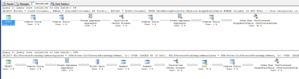

…………The results in Figure 2 are a powerful illustration of one of the weaknesses of the Jarque-Bera Test, i.e. its lack of scaling. The higher the values of the column accumulate in the internal calculations, the larger the test results may be; that is why the 209 rows of the LactateDehydrogenase column had much higher skewness and kurtosis scores than the results for Column1 and Column2 of the Higgs Boson table, yet had a Jarque Bera score that was several orders of magnitude smaller. I’m sure that by now some statistician has developed a scaling mechanism to get around this problem, but I question whether it is worth it for our purposes, for “…it is not without weakness. It has low power for distributions with short tails, especially for bimodal distributions. Other authors have declined to include its data in their studies because of its poor overall performance.”[7]  The latter wasn’t as much of an issue as expected in this example, but another problem frequently encountered in the last couple of tutorial series reared its head again: the lack of hard-and-fast cut-off points. I couldn’t find a clear winner among the competing criteria for when the Jarque-Bera stat disqualifies a dataset from being Gaussian (although that doesn’t mean one doesn’t exist, given that I lack experience with this field). They seem to all boil down to “rules of thumb,” out of those I’m most inclined to favor M.G. Bulmer’s, that skewness values beyond -1 or +1 are highly skewed, those within 0.5 of zero are pretty much symmetric and the rest are moderately skewed.[8]
…………It may be that we are better off without such hard limits though, given that they limit us to simplistic either-or choices. Confidence intervals are another common way of forcing the same kind of choice, when there might not be a real crying need for such a limit. If we use a continuous measure, we can ask questions about how close a dataset comes to a particular distribution, such as the Gaussian bell curve, but we lose all of that flexibility when we resort to arbitrary cut-off criteria. This is a problem we’ll probably see again as we work our way through the whole menagerie of goodness-of-fit tests, some of which blindly affix labels like “normal” and “not normal” in an almost manic depressive, all-or-nothing way. It’s always good to keep in mind that when we assign labels and test results in this way on a simple pass/fail basis, or perform binning and banding on the values within them, we’re sacrificing a lot of information. For our purposes, we’d probably be better of preserving the skewness and kurtosis values as measures of how skewed or kurtic a dataset is, as well as how normal it might be, rather than tossing out all the insights and details the full numbers provide. Skewness and kurtosis aren’t as useful in resolving the usual chicken-and-egg dilemma that accompanies outlier detection and goodness-of-fit testing, because we can’t determine whether or not a dataset follows a distribution closely but has too many outliers, or if those outliers signify that a different distribution is a better match. Yet they do occupy a substantial niche in the matrix of use cases I hope to develop for goodness-of-fit, as I did for outlier detection methods in my last mistutorial series. They’re simple enough for a layman to understand and easy to visualize, plus they represent really effective measures of the shape of a dataset, aside from whether or not that shape is applicable to goodness-of-fit testing. This makes them useful in their own right as primitive forms of data mining, in a sense. I’m not as enthused about the Jarque-Bera Test though, because it requires extra computational effort in order to derive results that lack adequate scaling, interpretation criteria and statistical power, even when implemented flawlessly by better programmers than myself. It may very well have valid uses in ordinary statistical applications, but its range of usefulness may be more constrained in the realm of databases servers and Big Data. Perhaps D’Agostino’s K-Squared Test, an alternative goodness-of-fit measure also built upon skewness and kurtosis, will prove more useful that the Jarque-Bera Test in next week’s article.

[1] See the Wikipedia page “Normality Test” at http://en.wikipedia.org/wiki/Normality_test

[2] See National Institute for Standards and Technology, 2014,  “1.3.5.11 Measures of Skewness and Kurtosis,” published in the online edition of the Engineering Statistics Handbook. Available online at http://www.itl.nist.gov/div898/handbook/eda/section3/eda35h1.htm

[3] Brown, Stan, 2012, “Measures of Shape: Skewness and Kurtosis,” published Dec. 27, 2012 at the Tompkins Cortland Community College website. Available online at http://www.tc3.edu/instruct/sbrown/stat/shape.htm .

[4] See Brown, Stan, 2012.

[5] I derived this code from the formulas at Brown’s webpage and the Wikipedia entry “Jarque-Bera Test” at http://en.wikipedia.org/wiki/Jarque%E2%80%93Bera_test

[6] For example,  see the thread posted by the user named ipadawan on Oct. 13, 2011 in the CrossValidated forums, titled “Appropriate Probability Threshold for Jarque-Bera Test,” which is available online at the web address http://stats.stackexchange.com/questions/16949/appropriate-probability-threshold-for-jarque-bera-test

[7] See the Wikipedia entry for “Normality Test” again, at http://en.wikipedia.org/wiki/Normality_test

[8] I’m paraphrasing Brown, 2012, who cites Bulmer, M. G., 1979, Principles of Statistics. Dover Publication: New York. I also agree with Brown when he says that “… GraphPad suggests a confidence interval for skewness….I would say, compute that confidence interval, but take it with several grains of salt — and the further the sample skewness is from zero, the more skeptical you should be.” I have no issue with GraphPad, which I’ve never used before, but am not inclined to much stock in hard confidence intervals anyways.