In the previous post I looked into some very basic and common measures of descriptive statistics – mean, median and mode, and how to derive these using T-SQL, R as well as a combo of the two in SQL Server 2016. These measures also called measures of ‘Central Tendency‘. In this post am going to describe some measures called ‘Measures of Dispersion‘. Dispersion refers to how much the said value differs from the average and how many such values are distributed around the average.

Below are 4 very common measures of dispersion –

1. Range
2. Inter-Quartile Range
3. Variance
4. Standard Deviation

The first and most common measure of dispersion is called ‘Range‘. The range is just the difference between the maximum and minimum values in the dataset. It tells you how much gap there is between the two and therefore how wide the dataset is in terms of its values. It is however, quite misleading when you have outliers in the data. If you have one value that is very large or very small that can skew the Range and does not really mean you have values spanning the minimum to the maximum.

To lower this kind of an issue with outliers – a second variation of the range called Inter-Quartile Range, or IQR is used. The IQR is calculated by dividing the dataset into 4 equal parts after sorting the said value in ascending order. For the first and third part, the maximum values are taken and then subtracted from each other. The IQR ensures that you are looking at top and near-bottom ranges and therefore the value it gives is probably spanning the range.

A more accurate calculation of dispersion is called Variance. Variance is the average of the difference between each value and the mean, divided by the number of values. When your dataset is comprised of an entire population the number of values are the total number of values, but when it is comprised of a sample, the number of values are deducted by 1 to ensure a statistical adjustment. The larger the variance, the more widespread the values are.

The last measure of dispersion am going to look into in this post is Standard Deviation.The Standard Deviation is the square root of the variance. The smaller the standard deviation, the lesser is the dispersion around the mean. The larger, the greater.

The higher the values of variance and standard deviation – the more skewed your data is and the less likely it is to lend itself to any real statistical analysis or even forecasting or predictive reporting.

I used the same data set that I did in the earlier post to run queries for this. Details on that can be found here.

Using T-SQL:

Below are my T-SQL queries to derive range, inter quartile range, variance and standard deviation. I was surprised to find that T-SQL actually has a built in function for variance, which makes it very easy. Was not sure why this particular function would exist when the vast majority of other statistical functions don’t, but makes sense to use it since it does

–Calculate range of the dataset
SELECT MAX(AGE) – MIN(AGE) as Range FROM [dbo].[WHO_LifeExpectancy]

–Calculate Interquartile range of the dataset
SELECT MAX(QUARTILEMAX) – MIN(QUARTILEMAX) AS INTERQUARTILERANGE
FROM
(SELECT QUARTILE, MAX(AGE) AS QUARTILEMAX FROM (SELECT NTILE(4) OVER ( ORDER BY Age ) AS Quartile ,
Age FROM [dbo].[WHO_LifeExpectancy]) A
GROUP BY QUARTILE HAVING QUARTILE = 1 OR QUARTILE = 3) A

–Calculate variance of the datasest
SELECT VAR(Age) AS VARIANCE FROM [dbo].[WHO_LifeExpectancy]

–Calculate standard deviation of the dataset
SELECT SQRT(VAR(Age)) AS STDDEV FROM [dbo].[WHO_LifeExpectancy]

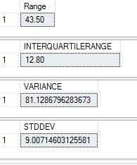
Results are as below:

Using R:

The R script to do the exact same thing is as below. None of these calculations require anything more than calling a packaged function in R, which is why it is usually the preferred way to do it.

#load necessary libraries and connect to the database
install.packages(“RODBC”)
library(RODBC)

cn <- odbcDriverConnect(connection=”Driver={SQL Server Native Client 11.0};server=MALATH-PC\\SQL01;database=WorldHealth;Uid=sa;Pwd=<password>”)
data <- sqlQuery(cn, ‘select age from [dbo].[WHO_LifeExpectancy] where age is not null’)

#Get range
agerange <- max(data)-min(data)
agerange

#Get Interquartile Range
interquartileagerange <- IQR(unlist(data))
interquartileagerange

#Get Variance
variance <- var(data)
variance

#Get Standard Deviation
stddev <- sd(unlist(data))
stddev

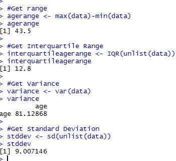
The results you get, almost exact matches to what T-SQL gave us:

3. Using R function calls with T-SQL

Now the last part , where we call the R script via T-SQL. We have to make small changes to the script – the ‘cat’ function to concatenate results, /n to introduce a carriage return for readability and removing the ‘unlist’ that native R needs because of how R structures data it reads directly from SQL . But for this the math is exactly the same.

 — calculate  simple dispersion measures
EXEC sp_execute_external_script
@language = N’R’
,@script = N’ range <-max(InputDataSet$LifeExpectancies)-min(InputDataSet$LifeExpectancies)
cat(“Range”, range,”\n”);
InterquartileRange <-IQR(InputDataSet$LifeExpectancies)
cat(“InterQuartileRange”, InterquartileRange,”\n”);
variance <-var(InputDataSet$LifeExpectancies)
cat(“Variance”, variance,”\n”);
stdeviation <-sd(InputDataSet$LifeExpectancies)
cat(“StdDeviation”, stdeviation,”\n”);’
,@input_data_1 = N’SELECT LifeExpectancies = Age FROM [WorldHealth].[dbo].[WHO_LifeExpectancy];’
;

And the results, exactly the same as the two above:

It has been fun so far doing this in 3 different ways and getting the same results. But as we go into more advanced statistics it will not be that simple. It will, however, definitely help us understand how far we can push statistical math with T-SQL, how easy and simple it is with R, and what can/cannot be done in the first version of calling R from within T-SQL. I can’t wait to play with it further and blog as I go along.

Thank you for reading.