I started my re-discovery of statistics with an introduction here. This second post is about descriptive statistics – very basic, simple statistics you begin with as a learner. Descriptive Statistics are also called Summary Statistics and serve to describe/summarize the data. They allow you to understand what the data is about and get a feel for its common features. There are two types of descriptive statistics

1. Measures of Central Tendency – for example, mean, median and mode.
2. Measures of Dispersion – or variation from Central Tendency such as standard deviation, interquartile range and so on.

You can figure out minimum and maximum values, outliers, average and most frequently occuring values with descriptive statistics. It takes you no further than that – it is not for deeper diagnostics of data, predictive or prescriptive analytics – but it is where you begin with in terms of understanding your data. In this post I took 5 very basic measures of descriptive statistics in category 1 for my specific measure – which is life expectancy across the globe.

1. Minimum life expectancy
2. Maximum life expectancy
3. Mean or Average life expectancy
4. Median or Central/mid point value of life expectancy
5. Mode or most common life expectancy.

It is easy to understand what are minimum and maximum values.They help you understand how wide the data set is. Some people also look at number of nulls in the dataset.
Mean or average is the sum of all values divided by number of values. Mean is very commonly used but does a poor job when there are outliers in the data such an unsually large or small value that can skew the average value.
Median is what you see as mid-point on a sorted scale of values. In other words median is the physical center of the data.Since median is not mathematically based it is rarely used in calculations. It does help with outliers better than mean does.
Mode is the most common value – very useful when you need to know to understand what are the values that occur most frequently. Mode can be used on nominal and ordinal data, hence it is the most commonly used measure of central tendency. There can be more than one mode in a sample.

The formulas to derive at these values are relatively simple – I tried them using both T-SQL and R, and also calling the R script via SQL. T-SQL is not really the best tool for statistical analysis, although it is useful for a beginner to get started.R are on the other hand has built-in functions for most of this.

With R integration into SQL Server 2016 we can pull an R script and integrate it rather easily. I will be covering all 3 approaches. I am using a small dataset – a single table with 915 rows, with a SQL Server 2016 installation and R Studio. The complexities of doing this type of analysis in the real world with bigger datasets involve setting various options for performance and dealing with memory issues – because R is very memory intensive and single threaded.

My table and the data it contains can be created with scripts here. For this specific post I used just one column in the table – age. For further posts I will be using the other fields such as country and gender.

Using T-SQL:

Below are my T-SQL Queries to get minimum, maximum, mean and mode.  The mode is rather difficult using T-SQL. Given how easy it is do with R, I did not spend a lot of time on it. How to arrive at the mode of a dataset using T-SQL has been researched well and information can be found here for those interested.

SELECT MIN(age) AS [MINIMUM-AGE],MAX(age) AS [MAXIMUM-AGE],
ROUND((SUM(age)/COUNT(*)),2) AS MEANAGE FROM [dbo].[WHO_LifeExpectancy]
WHERE AGE IS NOT NULL
SELECT TOP 1 AGE AS MODE FROM [dbo].[WHO_LifeExpectancy]
GROUP BY AGE
ORDER BY count(*) DESC

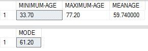
The results I got were as below:

Using R:

I downloaded and installed R Studio from here. The script should work just the same with any other version of R.

Before running the actual functions to get results, one has to load up the right libraries in R and connect to the database, then load the table contents into what is called a dataframe in R.Below commands help us do that.

install.packages(“RODBC”)
library(RODBC)

cn <- odbcDriverConnect(connection=”Driver={SQL Server Native Client 11.0};server=MALATH-PC\\SQL;database=WorldHealth;Uid=sa;Pwd=<password>”)

data <- sqlQuery(cn, ‘select age from [dbo].[WHO_LifeExpectancy] where age is not null’)

The data in my table is now in a dataframe called ‘data’ with R. To run statistical functions I need to ‘unpivot’ the dataframe into a single vector, and I have to use the ‘unlist‘ function in R for that purpose. When I run the R script via SQL, this is not necessary as it reads directly from the SQL tables. The R script i used to get the values is as below.

# Calculate the minimum value of data
minvalue<- min(unlist(data))
cat(“Minimum life expectancy”, minvalue)

#Calculate the maximum value of data
maxvalue<-max(unlist(data))
cat(“Maximum life expectancy”, maxvalue)

# Find mean.
data.mean <-mean(unlist(data))
cat(“Average Life Expectancy”, data.mean)

#Find mode
# Create the function.
getmode <- function(v) {
uniqv <- unique(v)
uniqv[which.max(tabulate(match(v, uniqv)))]
}

# Calculate the mode using the user function.
data.mode <- getmode(unlist(data))
cat(“Most common life expectancy”, data.mode)

data.median<-median(unlist(data))
data.median

Note that aside from mode all the rest are built-in functions in R. I borrowed the code for mode from here (the cool thing about R is the huge # of pre written scripts to do just about anything).

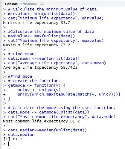
The results  I got are as below:

To be noted that the values of max, min, mean and mode are exactly the same as what we got from T-SQL which means this is correct.

3. Using R function calls with T-SQL

Details on configuration needed to use R within SQL Server are explained here.

The last and final step was to try the same script, without certain R specific commans such as ‘unlist’ to unlist the dataframe, and ‘cat’ to display concatenated results.  The scripts are as below. The first one is the call to basic statistics and the second is to get the mode. I separated the function for mode into a script in itself as it was multiple lines and hard to include within same call.

EXEC sp_execute_external_script
@language = N’R’
,@script = N’minvalue <-min(InputDataSet$LifeExpectancies);
cat(“Minimum life expectancy”, minvalue,”\n”);
maxvalue <-max(InputDataSet$LifeExpectancies);
cat(” Maximum life expectancy”, maxvalue,”\n”);
average <-mean(InputDataSet$LifeExpectancies);
cat(” Average life expectancy”, average,”\n”);
medianle <-median(InputDataSet$LifeExpectancies);
cat(” Median Life Expectancy”, medianle,”\n”);
‘
,@input_data_1 = N’SELECT LifeExpectancies = Age FROM [WorldHealth].[dbo].[WHO_LifeExpectancy];’
;

EXEC sp_execute_external_script
@language = N’R’
,@script = N’getmode <- function(v) {
uniqv <- unique(v)
uniqv[which.max(tabulate(match(v, uniqv)))]
};
modele <- getmode(InputDataSet$LifeExpectancies);
cat(” Most Common Life Expectancy”, modele);
‘
,@input_data_1 = N’SELECT LifeExpectancies = Age FROM [WorldHealth].[dbo].[WHO_LifeExpectancy];’
;

Other than a slight variation in mode , which i suspect is because of decimal rounding issues, the results are exactly the same as what we got via TSQL and R Studio.

In the next post I am going to deal with measure of dispersion. Thank you for reading and do leave me comments if you can!