This test is an extension of the Chi Square test I blogged of earlier. This is applied when we have to compare two groups over several levels and comparison may involve a third variable.

Let us consider a cohort study as an example – we have two medications A and B to treat asthma. We test them on a randomly selected batch of 200 people. Half of them receive drug A and half of them receive drug B. Some of them in either half develop asthma and some have it under control. The data set I have used can be found here. The summarized results are as below.

To understand this data better, let us look at a very important statistical term – Relative Risk .It is the ratio of two probabilities.That is, the Risk of patient developing asthma with Medication A/Risk of patient developing asthma with medication B. In this case the risk of a patient treated with Drug A developing asthma is 56/100 = 0.56. Risk of patient treated with drug B developing asthma is 32/100 = 0.32. So the relative risk is 0.56/0.32 which is 1.75.

Let us assume a theory/hypothesis then, that there is no significant difference in developing asthma from taking drug A versus taking drug B. Or in other words, that comparative relative risk from the two medications is the same, or that their ratio is 1. We can test this hypothesis using Chi Square test in R. (If you want the long winded T-SQL way of doing the Chi Square test refer to my blog post here. The goal of this post is to go further than that so am not repeating this using T-SQL, just using R for this step).

mymatrix3 <- matrix(c(56,44,32,68),nrow=2,byrow=TRUE)
colnames(mymatrix3) <- c("Yes","No")
rownames(mymatrix3) <- c("A", "B")
chisq.test(mymatrix3)

Since the p value is significantly less than 0.05, we can conclude with 95% certainty that the null hypothesis is false and the two medications have different effects, not the same.

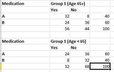
Now, let us take it one step further. Inspection of the data reveals that people selected randomly for the test fall broadly into two age groups, below 65 and over or equal to 65. Let us call these two age groups 1 and 2. If we separate the data into these two groups it looks like this.

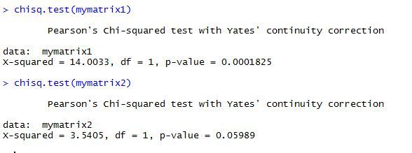
Running the chi square test on both of these datasets, we get results like this :

mymatrix1 <- matrix(c(32,8,24,36),nrow=2,byrow=TRUE)
colnames(mymatrix1) <- c("Yes","No")
rownames(mymatrix1) <- c("A","B")
chisq.test(mymatrix1)
mymatrix2 <- matrix(c(24,36,8,32),nrow=2,byrow=TRUE)
colnames(mymatrix2) <- c("Yes","No")
rownames(mymatrix2) <- c("A", "B")
myarray <- array(c(mymatrix1,mymatrix2),dim=c(2,2,2))
chisq.test(mymatrix2)

In the second dataset for people of age group < 65, we can see that the p value is greater than 0.05 thus proving the null hypothesis right. In other words, when the data is split into two groups based on age, the original assumption does not hold true. Age, in this case, becomes the confounding variable or the variable that changes the conclusions we draw from the dataset. The chi square test shows results that take into account the age variable. These results are not wrong but do not tell us if the two datasets are related for -specifically- for the the two variables we are looking for – drug used and nature of response.

To test for the independence of two variables and mute the effect of the confounding variable with repeated measurements, the Cochran-Mantel-Haenszel test can be used. If you  have a matrix as below , the formula for x-squared/pi value for this test is

The above image is used with thanks from the book Introductory Applied Biostatistics.

Using T-SQL: I used the same formula as the textbook, only added the correction of 0.5 to the numerator, since R uses the correction automatically and we want to compare results to R.(Disclaimer: To be aware that I have intentionally done this step-by-step for the sake of clarity, and not tried to optimize T-SQL by doing it shortest way for this. It is my humble opinion that these calculations are best done using R – T-SQL is a backup method and a good means to understand what goes behind the formula, nothing more.)

declare @Batch1DrugAYes numeric(18,2), @Batch1DrugANo numeric(18,2), @Batch1DrugBYes numeric(18, 2), @Batch1DrugBNo numeric(18, 2)
declare @Batch2DrugAYes numeric(18,2), @Batch2DrugANo numeric(18,2), @Batch2DrugBYes numeric(18, 2), @Batch2DrugBNo numeric(18, 2)
declare @xsquared numeric(18, 2), @xsquarednumerator numeric(18, 2), @xsquareddenom numeric(18,2 )
declare @totalcount numeric(18, 2)
SELECT @totalcount = count(*) FROM [dbo].[DrugResponse] WHERE batch = 1
SELECT @Batch1DrugAYes = count(*) FROM [dbo].[DrugResponse] WHERE batch = 1 AND drug = 'A' AND response = 'Y'
SELECT @Batch1DrugANo = count(*) FROM [dbo].[DrugResponse] WHERE batch = 1 AND drug = 'A' AND response = 'N'
SELECT @Batch1DrugBYes = count(*) FROM [dbo].[DrugResponse] WHERE batch = 1 AND drug = 'B' AND response = 'Y'
SELECT @Batch1DrugBNo = count(*) FROM [dbo].[DrugResponse] WHERE batch = 1 AND drug = 'B' AND response = 'N'
SELECT @Batch2DrugAYes = count(*) FROM [dbo].[DrugResponse] WHERE batch = 2 AND drug = 'A' AND response = 'Y'
SELECT @Batch2DrugANo = count(*) FROM [dbo].[DrugResponse] WHERE batch = 2 AND drug = 'A' AND response = 'N'
SELECT @Batch2DrugBYes = count(*) FROM [dbo].[DrugResponse] WHERE batch = 2 AND drug = 'B' AND response = 'Y'
SELECT @Batch2DrugBNo = count(*) FROM [dbo].[DrugResponse] WHERE batch = 2 AND drug = 'B' AND response = 'N'
SELECT @xsquarednumerator = ((@Batch1DrugAYes*@Batch1DrugBNo) - (@Batch1DrugANo*@Batch1DrugBYes))/100
SELECT @xsquarednumerator = @xsquarednumerator + ((@Batch2DrugAYes*@Batch2DrugBNo) - (@Batch2DrugANo*@Batch2DrugBYes))/100
SELECT @xsquarednumerator = SQUARE(@xsquarednumerator-0.5)
SELECT @xsquareddenom = ((@Batch1DrugAYes+@Batch1DrugANo)*(@Batch1DrugBYes+@Batch1DrugBNo)*(@Batch1DrugAYes+@Batch1DrugBYes)*(@Batch1DrugANo+@Batch1DrugBNo))/(SQUARE(@TOTALCOUNT)*(@totalcount-1))
SELECT @xsquareddenom = @xsquareddenom + ((@Batch2DrugAYes+@Batch2DrugANo)*(@Batch2DrugBYes+@Batch2DrugBNo)*(@Batch2DrugAYes+@Batch2DrugBYes)*(@Batch2DrugANo+@Batch2DrugBNo))/(SQUARE(@TOTALCOUNT)*(@totalcount-1))
--SELECT @xsquareddenom
--SELECT @xsquarednumerator,@xsquareddenom
SELECT 'Chi Squared: ', @xsquarednumerator/@xsquareddenom

We get a chi square value of 17.17. With T-SQL it is hard to take it further than that, so we have to stick this value into a calculator to get the corresponding p-value. The P-Value is 3.5E-05. The result is significant at p < 0.05. What this means in lay man terms is that the two datasets have differences that are statistically significant in nature and that the null hypothesis that says they are the same statistically is false.

Trying to do the same thing in R is very easy –

mymatrix1 <- matrix(c(32,8,24,36),nrow=2,byrow=TRUE)
colnames(mymatrix1) <- c("Yes","No")
rownames(mymatrix1) <- c("A","B")
 
mymatrix2 <- matrix(c(24,36,8,32),nrow=2,byrow=TRUE)
colnames(mymatrix2) <- c("Yes","No")
rownames(mymatrix2) <- c("A", "B")
myarray <- array(c(mymatrix1,mymatrix2),dim=c(2,2,2))
mantelhaen.test(myarray)

Results are as below and almost identical to what we found with T-SQL. Hence the conclusion drawn is valid, that the two datasets are different regardless of age.

In the next post I will cover the calculation of relative risk with this method. Thank you for reading.