by Steve Bolton

                In last week’s installment of this amateur series of self-tutorials on SQL Server Data Mining (SSDM), we covered my least favorite of the nine algorithms Microsoft includes with the product. There is a right time and place for every tool, but the times and places where Association Rules is the appropriate one are quite narrow. Its limitations make it an oddball among the major data mining methods, in that it is not used to construct other algorithms, nor does it use the others as building blocks. Functionally, it has the most in common with Clustering, an algorithm which also groups similar items within a dataset together. Association Rules is not technically referred to as a segmentation algorithm, but the two data mining tools group items in a dissimilar yet somewhat complementary way. Association Rules identifies the most common relationships between specific states of a couple of input or predictable columns in a mining model, in a sort of brute force, bottom-up way that leads to many small groups. In contrast, Clustering use more sophisticated, top-down methods to partition datasets into a handful of large groups, in which different states of the same column may be present in the same cluster. The first usually results in small itemsets, such as specific states of three or four mining model columns, while the latter may group together tens of thousands of rows in a particular cluster. In relational terminology, there are 1:M columns in each Association Rules itemset but a 1:1 relationship between columns and states, while the relationships for both are 1:M with Clustering. This week’s algorithm has the added advantage that a distance is often implied between clusters based on how divergent their constituent rows (i.e. cases in SSDM terminology) are from each other, whereas in Association Rules itemsets can only be crudely compared and contrasted by the probability with which they appear together.

                Not only does Clustering entail far less danger of overfitting (the bogeyman of data mining, in which decreased performance is paired with information glut, in the form of cluttered or misleading results) but it can accept the two major Content types, Discrete and Continuous. Association Rules requires the latter Content type to be Discretized into buckets, which leads to loss of information content. In fact, Clustering is unique among the SSDM algorithms in that it does not even require you to identify a predictable column. The behavior with PredictOnly columns is a little different than usual, in that they are assigned values in a second pass over the training data based on the values in the clusters, rather than being used to form clusters themselves.[ii] This data mining method can be put to use in making predictions[iii], but this is not often done. That is one of the few broad applications where its utility is limited though. Association Rules is mainly useful for market basket analysis and recommendation engines, but Clustering is used for so many purposes in so many different industries that it is not possible to count all of the varieties of the algorithm in use today. The majority of the applications have this in common: they are instances of what is termed “unsupervised learning” in data mining lexicon, in which data is classified, without knowing the classifications or their properties in advance. It is well-suited to discovering previously unknown determinants of your dataset, which makes it an ideal starting point for research in many widely varied academic fields. Today, research on the algorithm is balkanized among many different fields for that reason, rather than being the exclusive domain of information theorists, mathematicians and statisticians. Its origins were also divided among several different academic disciplines between the 1950s and 1960s. The two names most commonly associated with its genesis are mathematician Hugo Steinhaus and Stuart Lloyd, a physicist in the Manhattan Project, who began publishing research on early variants of the algorithm in 1957.[iv] As mentioned earlier in this series, the origins of some of the other prominent mining algorithms were clouded by the uneven judgment of their inventors, who sometimes succumbed to junk science or sordid philosophes in fits of unreason. This was certainly not the case with Steinhaus, a Pole of Jewish ancestry who spent World War II in hiding, on the run in his homeland from the Nazis.[v] After the Soviet occupation of Poland he was forced to toil in obscurity behind the Iron Curtain, like Petr Hájek, Ivan Havel and Metodej Chytil, three Czechs who helped lay the groundwork for Association Rules in the mid-‘60s, as discussed in last week’s column.

               In addition to academic research, the clustering algorithm is quietly used in a wide range of applications that millions of American unwittingly encounter on a daily basis, like image data compression, optical character recognition (OCR), image grouping, computer vision and speech recognition.[vi] The algorithm can also be used in reverse to find oddball data that doesn’t fit normal patterns within a dataset, which can illuminate eccentric relationships or help identify outliers, i.e. values that can throw off measures of central tendency like averages. In some fields, such as “medical diagnostics, fraud detection, network security, anomaly detection, and computer immunology,” the whole point of Clustering might be to identify outliers.[vii] Data Mining with Microsoft SQL Server 2008, written by several former members of the Microsoft’s Data Mining Team, is not only a readable and indispensable tool for users of SSDM, but contains a brilliant explanation of how to use Clustering for anomaly detection.[viii] Even those DBAs who are strictly focused on the relational OLTP world could use it to identify bad data that needs to be cleansed. In other scenarios, it may be preferable to filter outliers out of a dataset before processing, or to limit them to a single cluster; how they are handled depends highly on the goals of a particular mining project.[ix]

               The types of problems the algorithm can be applied to are so vast that selecting the right means of Clustering becomes of central importance, especially since it is an “exploratory” algorithm that is designed to make a little more sense out of large quantities of relatively unknown data. As the DM Team puts it in their aforementioned book, “It is possible for people with particular domain expertise and a deep understanding of the data to create clusters in up to five or six dimensions, but modern data sets typically contain dozens (if not hundreds) of dimensions, leaving you with the impossible task of creating groupings when you can’t even conceive of the possible relationships between the attributes.”[x] On the other hand, the wide range of applications and large datasets it is designed to tackle also leave it open to one of the most dreaded terms in mathematics: “the curse of dimensionality.”[xi] Basically, several complications arise at an exponential pace as new dimensions are added to data, including the multiplication of irrelevant attributes, which seems to be a problem with other data mining algorithms as well. Certain Clustering methods, such as the popular K-Means method included in SSDM, have the additional difficulty in that their calculations imply distances between clusters, which quickly recede into a vague mass with higher dimensional problems. Perhaps the most dreaded acronym in mathematics is “NP,” which designates certain classes of problems which are particularly difficult to solve. K-Means is not among the most difficult class problems, NP-Complete (some of which may be logically impossible to solve with finite resources), but it is considered to be NP-Hard to prove that it has found the best possible solution (i.e. the “global optimum”) to particular Clustering problems, without taking the prohibitively expensive step of examining each and every solution. Both of these terms are bandied about frequently in the literature around Clustering algorithms, which indicates the high difficulty level of the problems that they are designed to cope with.

               Furthermore, “clustering is in the eye of the beholder.” These words from computer science Prof. Anil K. Jain, one of the gurus of Clustering, say it all.[xii] This data mining method is so useful that it has become ubiquitous, but that comes at a cost of diffuseness in defining what a cluster is. The answer to that question is basically determined by the type of Clustering method one chooses to use, since they all define the groups they create differently.  This is merely one a long list of “user dilemma” questions posed by Clustering, which are often answered by the choice of Clustering method, like how to validate clusters, which features to select when defining them, deciding whether or not to normalize the data, focusing on or discarding outliers and determining whether or not the data even has a tendency to cluster.[xiii] There is also a trade-off between Clustering methods, in that some of them operate better on certain types of data distributions, while others are conducive to building clusters of particular shapes. As Jain puts it so succinctly, these problems are compounded by the fact that “different clustering algorithms often result in entirely different partitions even on the same data.” Some Clustering methods, like K-Means, may create clusters even where there are none, because the data is uniformly distributed. Others may partition data in a particular way that is entirely valid, yet miss other equally valid partitions. For example, in one of his recently published papers Jain cites a particular study in which a particular Clustering experiment divided animals into mammals vs. birds based on one iteration in which their appearances were heavily weighted, but in another iteration in which their activities were heavily weighted, they were segmented on the lines of predators vs. non-predators.[xiv] Basically, the term Clustering covers several thousand disparate means of dividing datasets into distinct chunks based on the similarities of their constituent cases (i.e. rows, in the instance of our data). The selection of methods must be determined by the dataset and the goals of the data miners, since it will unavoidably affect the outcomes. It might even be logically impossible to develop a single Clustering method that fits every type of experiment imaginable. As Jain says,

           “The above discussion underscores one of the important facts about clustering; there is no best clustering algorithm. Each clustering algorithm imposes a structure on the data either explicitly or implicitly. When there is a good match between the model and the data, good partitions are obtained. Since the structure of the data is not known a priori, one needs to try competing and diverse approaches to determine an appropriate algorithm for the clustering task at hand. This idea of no best clustering algorithm is partially captured by the impossibility theorem [Kleinberg, 2002], which states that no single clustering algorithm simultaneously satisfies a set of basic axioms of data clustering.”[xv]

               All of these considerations are in addition to the usual trade-offs in terms of calculation performance and ease in visualizing the results. Luckily, the two Clustering approaches Microsoft has included in SSDM are very easy to visualize, as we shall see in a few moments, quite literally. They’re also among the most established and well-known varieties of Clustering methods, which makes performance tuning, cluster modification and interpretation of the results a little easier. K-Means and the Expectation Maximization (EM) methods iteratively apply their internal methods of dividing data over and over until the point is reached where no more information is being added to the mining model, so processing stops. I like to picture the process as wrapping a ball of yarn around an object until none is left, except that with clustering we are wrapping up several different objects, separated by a certain amount of space determined by the levels of similarity between them. The process might also be likened to the way that rain drops are formed by condensation of water vapor around minute particulates of dust. The way in which the two algorithms go about it differs somewhat though, which has an effect on the results returned. The object of the internal math of K-Mean is to assign data points to particular clusters by iteratively reducing the squared error of calculations of Euclidean geometric distance between them; EM assigns data points by iteratively calculating probabilities that they belong in a particular cluster, which may include discarding clusters and repeating processing if some are found to lack sufficient case support. K-Means explicitly implies distances between clusters, while the probabilities used in EM only imply distance in a less defined way. The “soft clustering” approach of EM has some advantages over the “hard clustering” techniques of K-Means, however, in that its data points can belong to more than one cluster and that its clusters can have a wider range of shapes, whereas data points are limited to a single cluster in K-Means, which tends to produce spherical groups of roughly the same size. I’ve seen several sources say that K-Means are ideal for Gaussian distributions (i.e. bell curves) but EM also assigns probabilities based on the same data distributions, so I’m not sure which of the two choices in SSDM would be ideal for that scenario.[xvi] K-Means might be preferred, however, if you have an explicit idea of the number of clusters your data ought to produce. Its drawbacks include a lack of clear starting points (i.e., the variable k) to being clustering, the inability of verifying whether or not a global optimum has been reached, sensitivity to skewing by outliers, lack of scalability and difficulty in analyzing certain irregular data shapes.[xvii] Users also have to specify the number of clusters in advance, which in some respects defeats the purpose of exploring unknown data.[xviii] The twin difficulties of identifying the best starting points and the proper number of clusters means it is best suited to being processed in multiple runs with different parameter settings.[xix] Although Microsoft deserves kudos for adding support for Discrete data to its version of K-Means (in contrast to other simpler, less versatile implementations of it), data of this Content type is of less practical use than with EM, because the probabilistic methods used to calculate it don’t have much in common with the distance-based calculations for Continuous data in K-Means.[xx] One serious limitation of Microsoft’s implementation is that the distances calculated by K-Means are not returned in the metadata returned by the Generic Content Tree Viewer. These can be retrieved by using prediction functions, according to the documentation in Books Online (BOL), but the Data Mining Extensions (DMX) language SSDM uses is an advanced topic that we won’t be tackling in this series until all nine algorithms have been introduced.

                Another advantage of EM over K-Means is that it requires less memory during processing and a maximum of one database scans, which may be why it “outperforms sampling approaches,” according to BOL. The documentation also says it “has the ability to use a forward-only cursor,” but I’m not sure if this referring to internal processing under the hood or in DMX queries; either way, I will never find out, because I haven’t used cursors in years due to a fatal allergy. The performance of both algorithms can also be enhanced by making wise choices between the scalable and non-scalable versions of both. In the former, SSDM loads 50,000 cases at a time and only reads additional batches of the same size if the mining models haven’t converged yet. In the latter, the datasets are loaded in one huge gobble. BOL advises that “Because it operates on a local buffer, iterating through the data is much faster, and the algorithm makes much better use of the CPU memory cache; EM is three times faster than non-scalable EM, even if all the data can fit in main memory. In the majority of cases, the performance improvement does not lead to lower quality of the complete model.”[xxi] Advantages like these may be why Microsoft chose 1 – Scalable EM as the default for the CLUSTERING_METHOD parameter, followed by 2 for Non-Scalable EM, 3 for Scalable K-Means and 4 for Non-Scalable K-Means. As we shall see, I didn’t see much of a performance drop when switching to the non-scalable means, probably because the datasets we’ve been using throughout these trials are relatively small, at least for Clustering applications, which seem to run a lot faster than certain other algorithms at any settings on the same data. The DM Team’s book says that “The scalable clustering framework was created to solve the problem of too little memory to maintain the entire case set in memory. However, if you have enough memory, you can set the SAMPLE SIZE parameter…to 0 to tell the algorithm to use as much memory as necessary.”[xxii] Most of the trials I ran only consumed about 1 of the 16 gigabytes of RAM on my poor beat-up development machine, which may explain why I saw little difference in processing time with any of the non-scalable means. Reducing the SAMPLE_SIZE to 10,000 improved processing time to 0:45 from roughly a minute or two on various other EM trials, while setting it to 0 also yielded a respectable time of 1:23 that was better than certain other trials. Setting it to 1,000, however, yielded the worst performance time of any of the 15 trials in Figure 1, at 6:26. Processing ran on just one of the six cores throughout most of the additional time. I’m going to go out on a limb and speculate that too low of a SAMPLE_SIZE can decrease performance in some scenarios, by forcing SSDM to process increased numbers of unnaturally small batches. Also note that if you accidentally set it between 0 and 100, as I did once on accident, SSDM will return an error message.

Figure 1: Trial Results for the Clustering Algorithm at Various Parameter Settings (click to enlarge)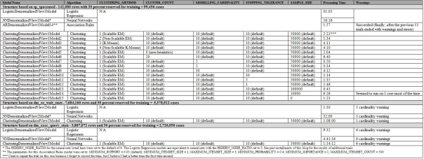

                 Many of the other variables mentioned above can also be explicitly controlled in SSDM. For example, the point where processing stops can be specified with the STOPPING_TOLERANCE parameter, which defaults to 10. According to BOL, when the change in cluster probabilities is below this number divided by the total number of cases, the model is believed to have converged and processing stops. A trade-off between performance and results is involved, with higher numbers leading to faster processing and looser clusters and lower numbers to slower processing and tighter clusters; the DM Team’s book advises that it can be set to 1 if you suspect in advance that you’re dealing with a “small data set or very distinct clusters.”[xxiii] All of the flavors of Clustering can be directed to begin their searches for place to condense at different data points, depending on the random number generated by the CLUSTER_SEED parameter, which defaults to zero. Setting it to different numbers may produce diverse clusters on the same data, particularly with K-Means. This makes it an ideal candidate to experiment with when we discuss model validation, a very important step in data mining, which we really can’t address adequately until we’ve covered all nine algorithms; for this reason I will save it for later in this series of amateur tutorials, along with other validation experiments I’m procrastinating on, like feeding different training data to the Neural Networks algorithm, as mentioned in A Rickety Stairway to SQL Server Data Mining, Algorithm 5: The Neural Network Algorithm. MODELLING_CARDINALITY is another parameter unique to Clustering which really shouldn’t be put off, since reducing below its default of 10 may cause SSDM to evaluate too few sample models during processing, thereby potentially improving performance at the cost of the quality of the results returned. Setting the number higher may of course have the reverse effect; keep in mind the omnipresent risk of overfitting when tweaking any of these parameters though, because the wrong settings may actually decrease both. The DM Team advises in its aforementioned book that “Typically you can reduce this by half without significantly impacting accuracy. If you are running the Enterprise or Developer edition of SQL Server 2008, each candidate model will be processed on separate threads, allowing you to take advantage of better hardware investments.”[xxiv] By default, SQL Server attempts to build 10 clusters, but the number can be explicitly set using the CLUSTER_COUNT parameter. Keep in mind that if SQL Server can’t build the number you specify, it “builds as many clusters as possible,” according to BOL. Setting it to 0 means that SQL Server tries to determine by itself the proper number of clusters to build, using a heuristic method that follows a curve that favors about 10 clusters. The DM Team book points out that “this heuristic is particularly important with discrete clustering, which tends to favor either very few or very many clusters, neither of which is particularly useful,” but it is difficult to tell from the documentation precisely how the presence of many Discrete columns will affect the number of clusters chosen.[xxv] This could be of importance with the third mining structure we’ve been working with, based on data returned by dm_exec_query_stats, which has many Discrete columns to indicate particular query texts, plan handles and the like.

               That mining structure has 3.8 million rows that took more than an hour to process, even with this fast algorithm, so I limited by experimentation with these parameters to the first mining structure, based on the 142,080 rows of data returned by sp_spaceused. See the first three posts in this series for a refresher on the schema we’ve been using throughout this series, which is based on more than three days of polling the dynamic management views (DMVs) dm_exec_query_stats, dm_io_pending_io_requests, dm_io_virtual_file_stats, dm_os_performance_counters, dm_os_wait_stats and sp_spaceused every minute. This deliberately created a disk bottleneck, so that I could study the IO subsystem better, while simultaneously providing a type of data for this series that is highly relevant to DBAs. We’ve already previously discussed parameters like MAXIMUM_STATES and MAXIMUM_INPUT_ATTRIBUTES which are also available in Clustering, so I won’t belabor those topics further. It is interesting to note, however, that there is there is no MAXIMUM_OUTPUT_ATTRIBUTES parameter in this algorithm, which I surmise has to do with the unique way in which predictable columns are handled. MAXIMUM_INPUT_ATTRIBUTES is relevant to the four methods of feature selection in SSDM, including the Interestingness Score, which is the only one Clustering makes use of, according to the documentation.[xxvi] I am a little unsure of this, however, because the other three methods that the documentation says it doesn’t use are all Bayesian, as described in A Rickety Stairway to SQL Server Data Mining, Algorithm 1: Not-So-Naïve Bayes. As we will see shortly, however, the root of each mining model returns a Bayesian Information Criterion, i.e. a Schwarz Criterion. Jain mentions this measure of information content is sometimes used to determine the number of clusters created by K-Means, but it is unclear from the documentation if this is the case in SSDM.[xxvii] We also don’t have room to do justice to the MINIMUM_SUPPORT parameter, which behaves a little differently with this algorithm, which may be why it was known by the different moniker of MINIMUM_CLUSTER_CASES in SQL Server 2005. Basically, it specifies that a cluster will be discarded unless it has the indicated number of cases. Setting this to numbers other than its default of 1 might make sense, for example, if you know that your clusters should logically have a certain minimum case support. This might be the case with our second mining structure based on dm_os_wait_stats, which returned near the maximum of 673 different wait types with each poll, so that it might make sense to partition our data into clusters near that minimum size to see if they divide into clusters based on the polling time. As always, a trade-off is involved with this parameter, because some of the clusters you filter out may include relevant data, if you’re not careful to set it properly. Keep in mind when setting it that the same case may occur in multiple clusters with EM but not in K-Means. Books Online also mentions the addition of an internal parameter called NORMALIZATION which is meant to control the collation of Z-scores, but I have not yet found a way to set it. Besides this, the only other variables we might concern ourselves with are the mining structure flags MODEL_EXISTENCE_ONLY and NOT NULL. Throughout this series we’ve ignored them though, since our data is not supposed to have nulls and turning our columns into a dichotomous choice between Missing and Existing would rob our data of meaning.

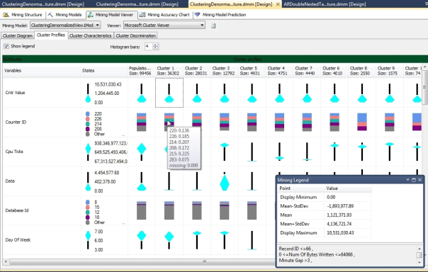
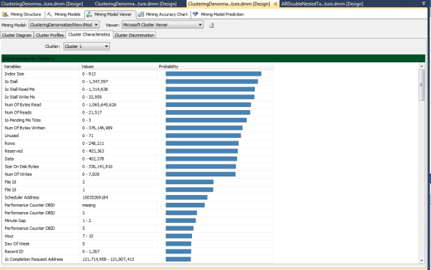
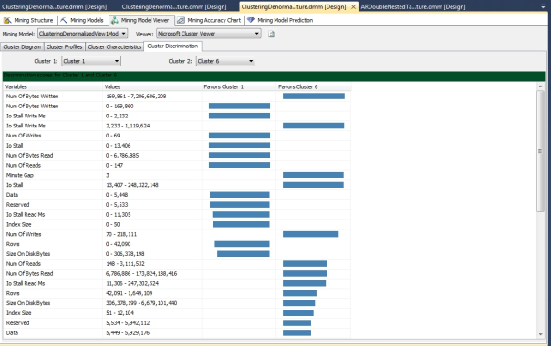
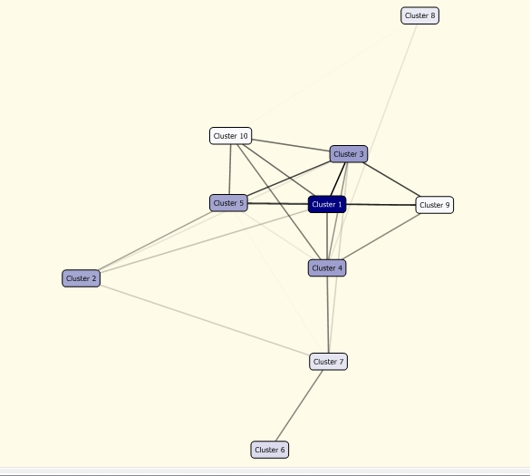
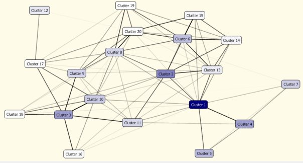
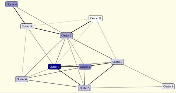
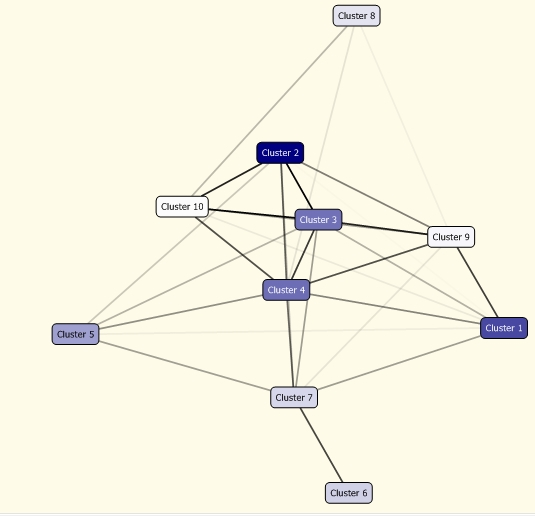
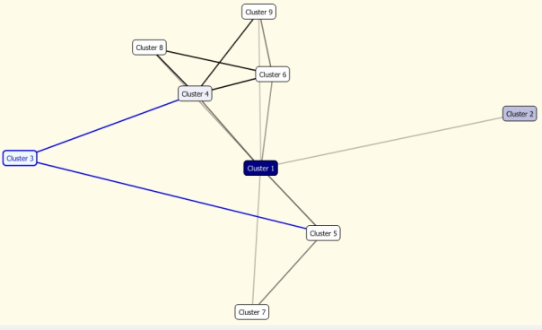
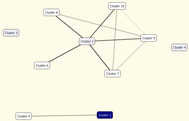
                The Cluster Diagram shows at a glance just how easy it is to visualize Clustering, at least in comparison to other algorithms. It operates much like the Dependency Network tabs introduced in previous posts, with the usual All Links slider to limit connections between the clusters by their statistical strength. The bluer a cluster is the, more members it has, while those with fewer members are shaded from grey to white in descending order of case support. Like with the Dependency Network tab, you can move the clusters around with your mouse. You can also right-click a cluster and select Rename Cluster… to specify a user-friendly name, but be aware that it won’t be persisted if you reprocess the model. The Cluster Profiles tab works much like the Attribute Profiles tab described in the Naïve Bayes Tutorial, except that it also includes Continuous columns with the minimum, maximum, mean, mean minus standard deviation and mean plus standard deviation displayed in the Mining Legend instead of the data distributions. As always, I’m not crazy about this tab, since it is difficult to digest all the diamond charts mixed together with histograms at a glance. The Cluster Characteristics tab also behaves like the Attribute Characteristics tab in Naïve Bayes, except that you can’t retrieve the probabilities by hovering your mouse over the blue bars. It is indispensable, however, in determining what cases belong to a particular cluster, which is isn’t readily evident with the other tabs. Cluster Discrimination operates like a stripped-down version of the Neural Network Viewer, in which one cluster is compared against another to see where a proportion of the cases for a particular attribute-value range fits best. The “Complement of Cluster” option can be selected from the dropdowns to see how a particular cluster compares against all of the values not included in it.[xxviii]

Figures 2-5: The Four Clustering Visualization Tabs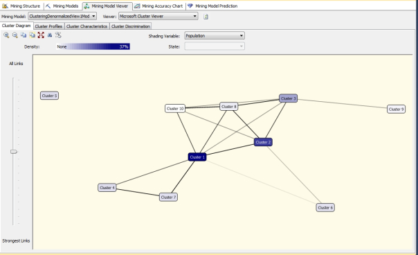

               If this isn’t enough information for us, we can dig down deeper into the data with the Generic Content Tree Viewer, which as always involves a tradeoff in the form of decreased legibility. In past articles I’ve discussed the challenges of SSDM’s common metadata format, which is a convenient way of representing the output of all nine algorithms that would ordinarily be akin to comparing apples and oranges. I look at it as a produce stand that can hold both, so to speak. The cost is that we have to sift through a denormalized table, whose rows can vary in meaning depending on the NODE_TYPE value, as well as the nested NODE_DISTRIBUTION table, whose rows can also vary in meaning depending on their VALUETYPE values. Furthermore, there are subtle differences in the meanings of the columns in this common format depending on the selected algorithm. Fortunately, interpreting this format is perhaps easier with Clustering than any other algorithm. As you can see in Figure 6, many of the columns are simply left blank or set to 0 or 1, or provide redundant like the name of the attribute. There are only two NODE_TYPE values, with one of those being the single model root node as usual. ATTRIBUTE_NAME and ATTRIBUTE_VALUE tell you the name of the attribute and the particular state that is the topic of that row,  while the standard codes we’ve worked with for most of the past few weeks are used for VALUETYPE, including 1 for Missing, 3 for a Continuous column, 4 for Discrete (and presumably, 5 for Discretized). The number of supporting cases, the probability of the attribute-value pair occurring and the variance are also listed in columns by the same names, as usual. The only difficult part of it might be interpreting the MSOLAP_NODE_SCORE, which BOL says returns a Bayesian Information Criterion score, as discussed earlier. I have not yet spotted a means to retrieve the Interestingness Scores, which are available in the model content of other data mining methods that use them, such as Linear Regression.

Figure 6: Metadata for Clustering (adapted from Books Online as usual)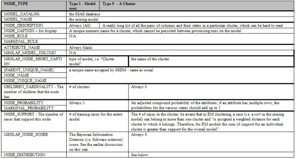

          The cluster with the most case support in the third mining structure, based on dm_exec_query_stats, was disconnected from the other nine clusters, which means it represented a group of highly distinct data. The Cluster Discrimination tab revealed dozens of states for specific Discrete measures like IOOffset, IOCompletionRequestAddress, IOuserDataAddress and SchedulerAddress, SQLHandleID tightly coupled with that cluster or its complement. The first group was strongly linked to values of 2 and 3 minutes for MinuteGap, an important measure I added to account for the unexpected increases in time between SQL Server Integration Services (SSIS) jobs during the data collection process. The complement strongly favored 1. A SQL Server internals or SSIS guru could probably easily use these figures to trace down the specific cause of this mysterious gap. The second structure, based on dm_os_wait_stats, had very weak links between its seven clusters, except for between the second and sixth clusters, which had just a few thousand rows between them out of the 5.4 million cases that were not reserved for training. This hints that the constituent attribute-value pairs represented outliers, previously unknown relationships or some other form of anomaly. This time the Cluster Discrimination tab revealed very high values for SignalWaitTimeMS, WaitingTasksCount, SizeOnDiskBytes, NumOfBytesWritten, IOStall, NumOfReads and IOStallReadMS in Cluster 2 and much lower values for many of the same values in its complement. This probably indicates that this group covered moments of particularly high IO pressure during the data collection process, possibly in terms of reads rather than writes, given that it was also associated with a NumOfWrites value of just 3.

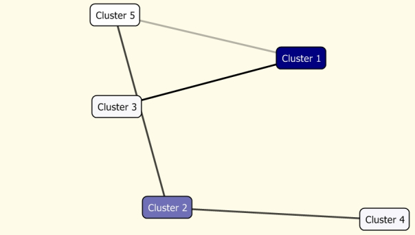
                The output for the smallest mining structure, based on sp_spaceused, took more labor to interpret because it varied depending on the parameters in Figure 1. As shown in Figures 7 through 15, the number and arrangements of clusters varied between eight different shapes for the 15 mining models created in this structure. The first illustration shows the identical results returned for the first two mining models, where EM and EM-Scalable were used with their default values. Likewise, in the second picture, identical results were returned for K-Means and K-Means scalable at their default values. The fifth, seventh, tenth, eleventh, twelfth and fifteenth mining models all had the same structure depicted in the third image. This was similar to the structure in the sixth picture, for the ninth mining model. The remaining illustrations depict the results for the sixth, eighth, thirteenth and fourteenth models, all of which were unique. The major determinants of these differences seemed to be setting the CLUSTER_COUNT to 20 with the sixth model, which therefore produced twice as many cluster, reducing the MODELLING_CARDINALITY to 2 and raising it to 30 in the eighth and ninth, and setting the SAMPLE_SIZE to 100,000 and 10,000 respectively with the thirteenth and fourteenth. The STOPPING_TOLERANCE didn’t seem to have much effect on the cluster shapes in this trial. The data returned by these various trials was useful in complementary ways. For example, the cluster with the most cases in the two K-Means trials had a complement with very high measures of IO Pressure like NumOfBytesRead, Unused, Data, Reserved and IndexSize associated with MinuteGap, in contrast to very low values for the first cluster. The first two EM models had a very high correlation between a MinuteGap of 3 in one small cluster, together with very high values for other measures of IO pressure like NumOfBytesWritten, NumOfReads, IOStall, IOStallReadMs and SizeOnDiskBytes, with very low values for the same measures associated with its complement. This cluster was also associated with a particular table in the Monitoring database that was continuously written to during the data collection process. It is possible that some read activity was going on as well, because like these numbers weren’t strongly associated with any measures of IO write activity either way, which is reminiscent of what we discussed above with one of the clusters in the second mining structure. It is entirely possible, looking back, that this small cluster represented moments in which I read from that particular table during data collection just to take some visual samples of how the process was going. That would be taboo during a real, live data collection endeavor, but in my experiment, I didn’t care about contaminating the data in this way because I deliberately wanted to create a disk bottleneck. Also note that the first two EM models and the first two K-Means models both produced strong, useful insights at a casual glance, but did so using entirely different sets of measures that were available to both. The most useful measures in the K-Means trials came from the columns returned by sp_spaceused, while in the EM ones they came from dm_io_pending_io_requests, which were joined together in the same view that the structure was built on. So SSDM automatically partitioned the data from different angles depending on the parameters we set, which led to different results which were nonetheless both useful and valid.

Figures 7 to 15: Cluster Diagrams for the 15 Models Based on sp_spaceused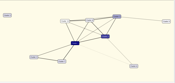

                If our results are this helpful at such a low performance cost using these two simple, well-known flavors of Clustering, it is intriguing to speculate on how much more might be revealed at minimal cost through other variants. As Jain has pointed out, there are already so many variations on the algorithm being put to productive use out in the wild that it is difficult even for an expert like him to track them all. Hierarchical clustering, for example, represents a whole set of Clustering methods that aren’t available in SSDM but which are useful for mining data that naturally follows a tier pattern; it is not derived from the Decision Trees algorithm we covered earlier in this series but is similar in many respects. Furthermore, new variants of Clustering are being developed all the time, including enhancements of older versions like K-Means. Some of these new forms of K-Means include two popular algorithms called ISODATA and FORGY, which sometimes also selects k through alternate methods like the Akaike Information Criterion.[xxix] New methods of Clustering based on data distribution densities are still being developed, such as DBSCAN and OPTICS, which don’t work well as well on Gaussian distributions as EM, which is in the same category of methods.[xxx] Other new variants are known by such colorful acronyms as CLARANS, BIRCH, CLIQUE, SUBCLU, DiSH and Eric.[xxxi] Much recent research has been focused on creating semi-supervised Clustering methods in order to improve the stability of the results, which can fluctuate greatly on similar datasets in some purely unsupervised scenarios.[xxxii] Canopy clustering is a method of particular interest, since it has a low performance impact and can be used to identify clusters before running more resource-intensive methods like K-Means and EM. It might thus be wise in some mining scenarios to perform canopy clustering on a cube or relational database, using your own code, in order to run SSDM trials more efficiently. We can add this to the growing list of preparation work that can be done in a cube or relational database prior to mining, along with determining the natural distributions of our data, computing variances and standard deviations and so on. More intensive preparation will be required to take the next step up our stairway, to a more limited variation on this family of data mining methods called Sequence Clustering. This algorithm first begins by Clustering data in much the same manner as we have in this article, but adds supplementary steps to place the clusters in a specific order, which requires the use of nested tables. Internally, it makes use of a common statistical building block called Markov chains, which are ironically often augmented by Clustering in Monte Carlo methods, a statistical building block which is beyond the scope of this series. Keep in mind that I’m posting this series in order to familiarize myself more with SSDM while simultaneously giving this incredibly useful product some badly needed free press, so if a data mining maven tells you that Sequence Clustering isn’t difficult to work with, listen to him instead. I have found it a challenge to work with in every SSDM application I’ve done to date though, to the extent that it has a steep learning curve similar to that of Association Rules. This is one of the reasons I’ve saved it for the tail end of this series, along with Time Series, another temporal mining algorithm.