by Steve Bolton
Anyone who has been following this series of self-tutorials has probably grown accustomed to me adding some kind of disclaimer about my shortcomings as a data miner. These blog posts are designed to simultaneously give the most under-utilized part of SQL Server some badly needed free press, as well as to make me think more intensively about SQL Server Data Mining (SSDM), as I try to upgrade my amateur-league skills to a more professional level. The data we’ve operated on throughout the series still essentially follows the outlines of the schema in post 0.2, which is taken from about three days of polling dm_exec_query_stats, dm_io_pending_io_requests, dm_io_virtual_file_stats, dm_os_performance_counters, dm_os_wait_stats and sp_spaceused every minute. I hoped to kill another bird with the same stone, so to speak, by deliberately creating a hard disk performance bottleneck using dynamic management views (DMVs) that are themselves disk-related, precisely because I don’t understand IO subsystems as much as I’d like to. All of these caveats still apply, but this week we’ll be tackling the one algorithm out of the nine included in SSDM that I actually have some uncommon prior experience with.
Like many other programmers, my first impressions about neural nets came from portrayals of artificial intelligence (A.I.) in science fiction films – many of which are imaginary instances of neural nets that mimic the structures of the human brain, as SSDM’s version does. Until I read a few books on the subject back in the 1990s, I was oblivious to the fact that neural nets had been put to real-world uses for a long time, such as eliminating static on phone lines; today, neural nets are put to uses that ordinary American benefit from routinely without knowing it, such as Optical Character Recognition (OCR) and credit card fraud detection. Neural nets are well-suited to fuzzy logic problems like these because they basically represent a fancy process of continual trial and error, in which interconnected nodes analogous to the human brain are assigned weights that are corrected in proportion to how far off their last answer was to a particular problem. They can have spectacular results for problems where imprecise answers are acceptable, which is often the case where definite solutions are not yet known, yet these strengths also make them poorly suited for problems where the right answer must be reliably given each time. For example, a hospital might gain live-saving insights into patient mortality that correlate medication data over several years, but a neural net might lead to mortality if used to adjust respirator functioning in real time. Because it is analogous to the human mind, it works well for some of the same problems that humans are adept at solving, but shares the same limitations all but a few prodigies like Srinivasa Ramanujan do when it comes to competing with computers at number-crunching. It can also be more resource-intensive than other data mining methods and is a really poor choice when it is crucial to understand why your algorithm spit back a particular results; it is not difficult to explain the architecture and functions that sustain a neural net, but explaining why the constituent neurons have particular weights is an arcane question akin to interpreting a man’s thoughts from a slice of his cerebellum.
Neural nets share some of the limitations of biological structures because they are analogous to them, but no matter how sophisticated they become, it is good to remember that they are just that: analogies. Despite the image Hollywood projects, they are a poor choice if you want to create intelligent life; if that is your goal, the simplest means yet known are to have a child. Computers with consciousness have become such a staple of the genre that the Wikipedia maintains a “List of Fictional Computers” that now has more than 500 entries, covering the film, television, paperback, comic and video game media, among others. Who could forget Arnold Schwarzenegger’s famous lecture in the film Terminator 2 on how his neural net brain learns from contact with humans? I hate to be a killjoy, but if given enough space I could provide a detailed argument that the archetypical sci-fi scenario of computers coming to life is physically possible, but not logically possible; furthermore, the Turing Test often cited as a litmus test of A.I. is yet another instance of very faulty philosophy being developed by a very talented mathematician (in this case, arguably the greatest cryptographer of all time).[ii] These are issues best left for other types of blogs, but suffice it to say that information content has nothing to do with consciousness or will; simply increasing processing speed or changing the architecture of our algorithms isn’t going to bring us one iota closer to creating life. That doesn’t mean, however, that neural nets aren’t capable of arriving at “good enough” conclusions to certain fuzzy logic problems, at speeds that no human mind could ever possibly match. As I have seen first-hand, the hype surrounding them is deserved, as long as they are limited to the right classes of tasks. We have barely scratched their potential for both good and evil. Fortunately, neural nets aren’t tainted with the kind of ignoble history that some of our algorithms have been, but as many sci-fi writers have pointed out, they could be put to ignoble uses in the future. Theoretically, you really could build a Skynet or Hal (the most famous examples of the old sci-fi chestnut, the machine gone mad) that could kill countless human beings through sloppy reasoning, if some future generation were foolish enough to abdicate its decision-making powers over matters that only humans ought to be trusted with. In fact, there has been loose but sincere talk within the Western intelligentsia over the last decade of developing cars that drive themselves, using technology that would almost certainly include neural nets, but this is merely a warning sign that these people have lost touch with reality. Neural nets are well-suited to fuzzy logic problems which overlap some of the same problems that the human mind is adept at solving, but no matter how good they get, they’re always going to make mistakes in ways that traditional computers don’t when solving straight-forward math problems. Some types of neural nets are even prone to catastrophically forgetting everything they have learned. If there is a one in ten thousand chance that a computerized driver might suddenly decide to swerve to the left on an off-ramp, or forget how to drive altogether, I think I’ll stick to bike paths. To put it bluntly, hare-brained schemes like this are most likely going to be the leading causes of death from A.I. in the next century rather than some child-like death machine like Joshua in the film War Games. As I have repeated many times throughout this series, data mining, like mathematics and the hard sciences, is a very powerful tool that is also very limited, in that it cannot be a substitute for good judgment. As long as these fields stay grounded in sound reasoning, they can be exceptionally beneficial to mankind, but the minute they depart from it, they merely add sophistication to falsehood. This must be kept in mind at all times when using SSDM or any other data mining tool: without the purely human capacity for rational, critical examination, the results can be simply unintelligible, or even dangerously misleading.
With that necessary note of caution out of the way, the bright side is that the potential benefits of neural nets could be quite substantial over the next century as long as they are applied to the right type of jobs: fuzzy logic problems where the solution is not known but wrong answers are occasionally acceptable. Out of the nine SSDM algorithms, this one is clearly best-suited to that class of problems and also the one with the most potential for future growth. For example, some the others we’ve surveyed, like Naïve Bayes or Decision Trees, might be useful in detecting relationships between certain carcinogens and increased rates of cancer; but for a really spectacular breakthrough, we’d have to look to neural nets. A properly designed net, for example, could conceivably cull all of the nation’s health data on cancer and spit back out a potential course of treatment human researchers would have never guessed, especially since people simply don’t have the processing capability to directly sift through vast amounts of data. And as I have seen first-hand, they can be crafted for more innocuous uses like playing games. I became interested in neural networks roughly a dozen years ago, when I was trying to teach myself Visual Basic 5 and 6 on an old Compaq with a 2 gigabyte hard drive. After skimming a book or two on the subject, I spent a few hours assembling a couple of different types of neural nets together to play the ancient Chinese game Go, which is featured often in the 1998 sci-fi film Pi.[iii] If it took a couple of hundred games or a few weeks of time for my best module to consistently defeat another that made simple random moves, I would have considered it a resounding success. You could imagine my surprise when my best A.I. module not only beat the random module right off the bat, but ended up shutting it out completely (a particularly difficult maneuver to pull off in Go) on the first day, within an average of about 10 games; every time I blanked out the data in the winning module and started the trial over, it consistently relearned how to shut out the random module after roughly the same interval. I immediately saw how powerful neural nets can be, even with no training data, very little time to train the net, a minimal learning curve on my part and archaic hardware that didn’t even have a quarter of the hard drive space of the MP3 player I use now.[iv] What I implemented with no formal training was in some respects fancier than what goes on under the hood in SSDM, so it shouldn’t be that difficult for other laymen to grasp how the SSDM implementation works. Microsoft’s version is not flexible enough to implement my experiment with hybrid neural nets, but it is still certainly among the best of the nine algorithms in terms of performance vs. the usefulness of the results, which were immediately apparent the first time I processed my data for this trial. It also has the added benefit of being able to simultaneously handle both of the most important Content types, Continuous and Discrete, which I elaborated on in A Rickety Stairway to SQL Server Data Mining, Part 0.0: An Introduction to an Introduction along with other basic topics like how to create a project and a Data Source View (DSV), etc. The Neural Networks algorithm seems to handle both more gracefully than the sort of shotgun marriage we see in Decision Trees, which creates separate regression and classification trees depending on the combination of Content types.
Ordinarily I would have saved Neural Networks for the final algorithm in our series, because of its complexity, the sophisticated nature of the problems it can solve and its immense potential, but I wanted to stick with the concept of statistical building blocks I touched on in A Rickety Stairway to SQL Server Data Mining, Part 0.1: Data In, Data Out. Basically, the Microsoft version is an extension of the mining method we covered last week in A Rickety Stairway to SQL Server Data Mining, Algorithm 4: Logistic Regression, with weighted nodes placed between the two layers of inputs and predictable outputs. Like Logistic Regression, it makes use of a common statistical method called Z-scores to put disparate ranges of inputs on a comparable scale; as detailed in the last tutorial, the method’s first building blocks are averages, which are used to construct variances, then standard deviations, followed by Z-scores. Logistic Regression is also, in turn, a refinement in some ways of Linear Regression, which is also a parent of Decision Trees; like these and several other SSDM algorithms, Neural Networks also depends upon Bayesian methods of feature selection akin to those outlined in A Rickety Stairway to SQL Server Data Mining, Algorithm 1: Not-So-Naïve Bayes. All of these algorithms have already been covered previously in this series and if you have a basic grasp of how they work, you should be able to understand how Microsoft’s implementation works sufficiently to get benefit out of it. Even without it, a quick discussion of how neural nets work in general should suffice. Bogdan Crivat, one of the heavyweights on Microsoft’s Data Mining Team before he moved on to Predixion Software, once posted in the Microsoft Data Mining Forum that “Microsoft Neural Networks is a standard single layer back propagation implementation. The model is presented at great detail in Christopher Bishop’s Neural Networks for Pattern Recognition book,” which I have not read but which is widely available for sale on the Internet.[v] Remember, one of the points of this series of self-tutorials is that you don’t need to have a formal background in statistics to get benefit from any of the nine SSDM algorithms; any DBA, even one working on OLTP rather than OLAP systems, can reap substantial benefits from them with only a moderate investment of time and energy. The more you know, the more benefit you will receive, but you don’t really need to know the equations that power neural nets to use them successfully, anymore than you need to know how to build your own combustion engine before learning to drive a car.
That being said, let me start off with a very simple equation that illustrates the storage potential of the human brain. The average brain has about 86 billion neurons, each of which has an average of 7,000 synaptic links to other neurons[vi]; do the math and you can see we’re already up into quadrillions of connections, which is quite a formidable storage capacity. Yet that is only the beginning, since we also have to factor in the relative strength of each electrical connection between neurons, which certainly helps the brain to encode information as well. We don’t really know how much of a change in voltage across synapses is required to affect the information content of neurons; if for argument’s sake it took only a few picovolts, then the range of numeric values for voltage that could encode information in a single synapse could be quite substantial. This is even before we get to the whole controversy over whether brains can use one of several hypothetical mechanisms to encode information using quantum states, in which case sci-fi A.I. will be out of the question before the advent of quantum computers.[vii] Neural nets are an analog of the human brain that combine all of these methods of information storage (save for the speculation on quantum states) through a similar method of weighted nodes that are connected to each other, much like neurons are linked through synapses. Ironically, the first neural nets were not merely copies of known structures within the brain, but served as a model for how neurons might hypothetically work. When neurophysiologist Warren McCulloch and logician Walter Pitts wrote the first research paper on neural nets back in 1943, the way in which neurons functioned was still a matter of speculation.[viii] Their research was modeled on electrical circuits, but one of the next major milestones came in the form of an algorithm developed in 1957 by Frank Rosenblatt of Cornell University. He theorized that information could be encoded by feeding a network of virtual neurons with the correct answers to a particular problem, then gradually changing the weights associated with each connection until they approximated the correct answer. The perceptron, as it is called, could only solve a limited range of problems because it had only two layers of neurons for the inputs and outputs, like Microsoft’s implementation of Logistic Regression. For example, it could solve simple AND as well as OR tasks, but not XOR problems. Information in this kind of “feed forward” network also moves in just one direction. Since then, refinement in neural nets have proceeded along several main lines, including experimentation with the activation functions used to alter the weights and changes in network topology. One of the key milestones in the latter was the development of multilayered networks in 1975, which made solutions to new ranges of problems, such as XOR, possible.
This kicked off a renewal in interest in the algorithm, which had faded following several setbacks in research.[ix] The activation functions used to correct errors in the network weights were also upgraded in this intermittent period, from the Hebb Rule proposed by psychologist Donald Hebb in 1949 to the least mean squares formula, or Delta Rule, developed by electrical engineering professor Bernard Widrow and his student Ted Hoff in the early ‘60s. The Widrow-Hoff rule, as it was also called, was not adequate for the new “back propagation” multi-layer networks postulated in 1986 by three separate groups of researchers, in which errors were filtered backwards from the output layer through the hidden layers to the inputs. This required an update to the Widrow-Hoff Rule called the Generalized Delta Rule. Unless you’re developing your own neural nets outside of SSDM, the important thing to remember is that all of these activation functions form a gradient of some kind; the trick is to find one that distributes the errors in a way that is most relevant for the particular kind of network you’re operating on, so that the nodes can learn from their mistakes. We’re skipping several other milestones in the history of neural nets, but one we ought to mention is the development of hybrid nets in 1982 by Brown University Professor Leon Cooper and two colleagues, which allowed different activation functions to be used at different points in a single net.[x] The SSDM implementation combines two separate functions, a hyperbolic tangent that constrains weights in the hidden layers to values on a Continuous scale between -1 and 1 and a sigmoid function that constrains the output layer to Continuous values between 0 and 1. I must confess some ignorance about the math behind each (even though I may have included them in my Go implementation years ago), but I know they’re both standard building blocks in neural networks. If you picture the process of feeding forward data and back propagating errors as a sort of wave (that might be more helpful to someone with a physics background) then sigmoid functions are particularly useful in smoothing out waves that might be too jagged, in a means crudely analogous to the way in which Logistic Regression smooths out the straight line relationships seen in Linear Regression. And as Books Online (BOL) points out, it is also useful for encoding probabilities.[xi] BOL also mentions that SSDM uses the conjugate gradient algorithm, which I am not familiar with, during the backprop phase. In a nutshell (as I understand it), the inputs and their probabilities are encoded and scaled using Z-scores, then their weights are summed and fed forward to the hidden layers, where the hyperbolic tangent function is applied on a scale between -1 and 1, so that negative weights inhibit connections to adjacent nodes and positive ones strengthen them. Then the results are fed forward to the output layer using the sigmoid function for smoothing, then the answer is compared against the desired results gleaned from the training set and the error is back propagated through the network using a conjugate gradient function.
The SSDM algorithm takes a lot of the grunt work out of developing your own neural nets, if you’re sticking to standard methods like backprop with sigmoid functions. The main drawbacks are that you can’t change the activation functions or the topologies, which means you can’t implement a wide range of other types of neural networks that have branched off from the original research. Among these are Kohonen networks, or self-organizing maps that mimic how the human eye encodes information; Hopfield nets, a content-addressable form of imitation memory (which are unfortunately prone to catastrophic forgetting) and simulated annealing, which is analogous to “heating” and “cooling” neurons into high and low energy states until they rest at an acceptably good answer. Boltzmann machines are another innovation that seems to combine elements of both Hopfield nets and simulated annealing, in which neurons are connected in a circular pattern rather than in a feed-forward network. Since I last read about them in the 1990s, the difficulties in scaling them to tackle larger datasets have apparently been overcome by the development of a new topology, in which a series of circular Boltzmann machines are stacked upon each other.[xii] I have put the flexibility to change activation functions and implement different topologies like this at the top of my SSDM wishlist for future versions of SQL Server. The current version of Neural Networks is already sufficiently powerful, however, to solve many types of problems in a more efficient manner than any of the other eight algorithms. When I ran the usual trials of our data through this particular data mining method, it returned some of the most interesting results to date, without the sort of performance hit we’d expect to pay to return the same quality of output with other algorithms.
The Neural Network algorithm has the same parameters as its stripped-down cousin, Logistic Regression, except for the addition of the crucial HIDDEN_NODE_RATIO, so we’ll focus our attention on that. As usual, we’ll leave the mining flags MODEL_EXISTENCE_ONLY and NOT NULL at their defaults since our data shouldn’t have nulls and ought not be reduced to a dichotomous choice between Missing and Existing states. The four standards means of feature selection are available with neural nets, but unlike with Decision Trees, we have no control over which of the four SSDM applies under the hood at any given time. For that reason, and the fact that we’ve already discussed them in previous articles, we’ll leave the ubiquitous MAXIMUM_INPUT_ATTRIBUTES and MAXIMUM_OUTPUT_ATTRIBUTES parameters alone as well. Not surprisingly, the same cardinality warnings were returned in both this week’s and last week’s trials when MAXIMUM_STATES was left at its default value of 100, at least when our neural nets were set up without hidden layers, so that they were equivalent to Logistic Regression. We’ve already played with that parameter in this past, however, so there’s no pressing need to revisit it, not when the HIDDEN_NODE_RATIO returned results strange enough to command our attention. As discussed in last week’s post, all of the nine algorithms have HoldoutSeed, HoldoutMaxPercent and HoldoutMaxCases properties that allow you to customize the training set for your mining structures somewhat. Logistic Regression and the Neural Network algorithm also have similar parameters like HOLDOUT_PERCENTAGE, HOLDOUT_SEED and SAMPLE_SIZE which allow you to customize training sets for individual mining models within a particular mining structure. This is because node training is a more important consideration with neural nets than other algorithms, and Logistic Regression is merely Microsoft’s version of the Neural Networks algorithm without the hidden layers. Ideally, we would compare the usefulness of results and performance of our neural nets against each other by tweaking these training parameters, but I need relevant material for a future post on Cross Validation and the Data Mining Accuracy tab, so I’ll save that discussion until some point after we’ve surveyed all nine algorithms. That gives us time in this week’s trials to delve into the HIDDEN_NODE_RATIO, which is multiplied by the square root of the number of input and output neurons multiplied, to give us the number of neurons in the interior layer. One aspect I’m still in the dark about is how many hidden layers SSDM adds and what effect, if any, this parameter has on that figure. At one point I misread the documentation and believed that this figure would also create an equivalent number of hidden layers, but on second glance that doesn’t appear to be the case. There’s no mention in BOL of additional layers being created, nor was there any evidence in the Generic Content Tree Viewer of any more than one hidden layer in any of the neural net models I created. If the number of layers did not increase in proportion to the HIDDEN_NODE_RATIO, that might lead to a lopsided topology, which might explain some of the squirrely results I received when messing with this parameter.
That is not to say that I was not pleased with the outcome. In fact, the models I built returned some of the most useful results to date at a lower cost of resources than I expected. RAM consumption never got above a gigabyte or so and IO pressure was next to nil during the processing of all the models and retrieval of their results. Unlike Decision Trees, which consumed all six of my cores throughout most of my trials with that algorithm, the neural nets I built seemed to hover between two and four – which freed up my computer for other activities, although I don’t think that would be a factor in a professional situation where we’d probably be working on a dedicated server. From what I understand, the term “overfitting” is not used with all data mining methods, but its twin dangers are basically the same in every algorithm: an increase in server resource consumption that also degrades the quality of the output, in the form of cluttered, nonsensical or misleading results. If overfitting were to occur in an SSDM neural net, the most likely culprit would be an excessively high HIDDEN_NODE_RATIO. I’ve seen overfitting with every other algorithm, but in this particular trial, I can’t say for certain that we precisely crossed that line. If anything, we entered the Twilight Zone, because the HIDDEN_NODE_RATIO had some unexpected side effects on the results that weren’t necessary deleterious.
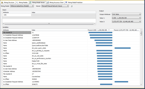
Before we get tangled up in the hidden layers of our neural nets, it would be helpful to put the anomalies into perspective by showing some examples of the really useful results that the algorithm returned right off the bat. As depicted in Figure 1, the Neural Network Viewer (which was introduced in last week’s column; refer to that for a refresher if necessary) immediately returned very strong links between several specific table names recorded by sp_spaceused and specific IOUserDataAddresses and FileHandleIDs with very high and low values for CntrValue, a measure in dm_os_performance_counters that corresponds to a performance counter value. The next obvious step in our workflow would be to correlate it with a specific CounterID, which is depicted in Figure 2, where we compare the same values against the unique identifier we’ve assigned to a particular performance counter. Ordinarily we might choose to leave the performance counter names as Text values in our data, but I assigned integer keys in the hopes that it might speed up processing of our mining models, so in this case we can look up #220 and see that it corresponds to the counter named Log Growths, which had really high counter values in association with the dm_exec_query_stats table we used to record the data from that particular DMV during the data collection process. Furthermore, IOCompletionRequestAddress 121645864 and IOUserDataAddress 15084414912 were also associated with the same values and IOUserDataAddress 148546358 strongly favored very low values. In all likelihood, this was due to sizeable, repeated transaction log growth during the collection process, particularly with dm_exec_query_stats, which was a major performance hog compared to other DMVs because it has many columns with potentially high values, such as columns featuring the full text of SQL queries. It is not surprising that the same DMV had values in the same range for five related counters, Data File(s) Size (KB)), Log File(s) Size (KB), Log File(s) Used Size (KB) and Percent Log Used. All of these except the CounterID corresponding to Log File(s) Used Size (KB) had high values in the same range for IOCompletionRequestAddress 121645864. The specific IOUserDataAddress 148546358 had very high values in that same range for Data File(s) Size (KB) but strongly favored the low range for Percent Log Used. I’m certain a seasoned SQL Server internals veteran could easily use such well-defined links to track down a specific performance issue. I’m still an amateur at that end of SQL Server – which is why I decided to use IO data for these trials – but I can say for certain that are among the strongest, most specific correlations returned by the algorithms we’ve surveyed to date. Quite useful correlations were returned for many other measures in the three mining structures we’ve been using in these trials. For example, I was puzzled for a minute when I saw that the wait stats SQLTRACE_PENDING_BUFFER_WRITERS and SQLTRACE_SHUTDOWN had really high values for IOStall in the second mining structure – until I remembered that I continually monitored the data collection process with a SQL Server Profiler trace, which I had sometimes had to restart due to the performance issues I deliberately created. Another important measure of IO pressure in the third mining structure was also strongly associated with very high and very low values for certain query texts, plan handles and other columns that could help us to quickly track down specific resource-gobbling queries.
Figures 1 and 2: Definite Performance Counter Correlations with Specific Tables and Data Addresses

Ordinarily I’d go into a little more detail on the strong, specific and very useful links that the algorithm returned, just to prove how valuable neural nets are, but I want to focus on a conundrum that arose during this week’s trials. In order to play with the HIDDEN_NODE_RATIO and see what kind of effect it had on performance, I ran trials with it at different settings on 10 different mining models in the smallest mining structure, which is based on the data returned by sp_spaceused during the collection process. Figure 3 shows the processing times for all of the models in this week’s trials, plus the results for the three mining models in last week’s post on Logistic Regression, which is equivalent to a perceptron without any hidden layers. For the most part, processing time increased in tandem with the number of hidden nodes, as well as by how many rows, columns and overall data each mining structure had. There were a few discrepancies in which processing time actually decreased a little as the HIDDEN_NODE_RATIO went up, but that might be explained by the fact that I was using my beat-up development machine for other activities at the same time; I was careful not to run any processor, memory or IO-intensive programs, but that doesn’t mean I didn’t have a momentary spike here or there when my eyes were turned away from the Performance Monitor in Windows. All in all the performance results were pretty much what we’d expect.
Figure 3: Performance Comparisons for the HIDDEN_NODE_RATIO Parameter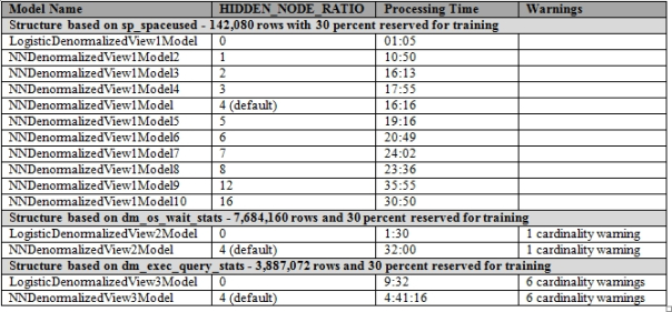
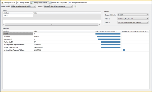
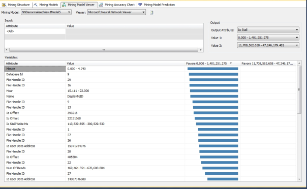
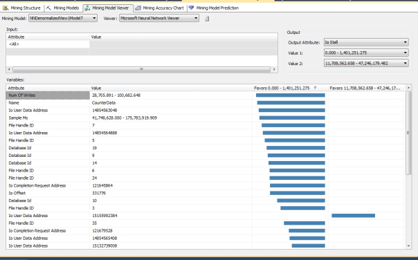
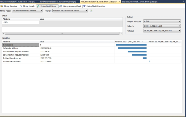
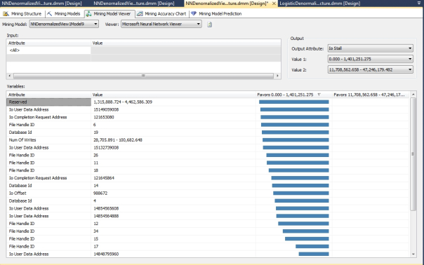
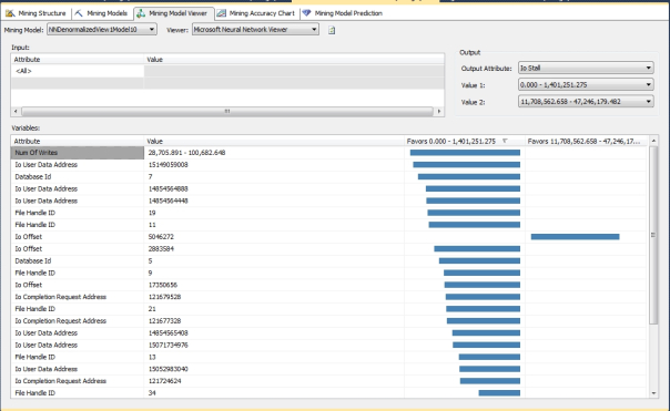
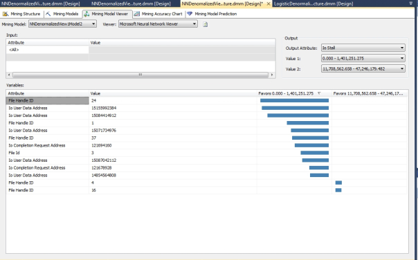
The same can’t be said for the correlations returned by the mining models based on sp_spaceused, which varied in an unpredictable fashion depending on the HIDDEN_NODE_RATIO. As you can see from Figures 4 through 13, the correlations to two specific ranges of IOStall values varied wildly from one model to the next, with just minor changes in this one parameter. I didn’t bother to post a screenshot of the third model because it didn’t return any correlations at all. If you look closely, even some of the graphs that appear similar at first glance actually reference specific input states that are very different from one model to the next. I can’t really classify this conundrum as an example of overfitting, because some of these results are actually relevant. Theoretically, we shouldn’t see this much variation from one iteration to the next merely because of the addition or subtraction of a few hidden nodes; it’s been a long time since I read the pertinent literature, but I don’t recall any reference to the results being dramatically altered like this, in such a seemingly random way. Ordinarily, the problem we’d have to watch out for with adding extra nodes is overfitting, i.e. expending a lot of processing power to get back meaningless or misleading results. In this case, it is almost as if the hidden layer bifurcated the correlations into different sets.
Figures 4-13: Disparate Results Depending on the HIDDEN_NODE_RATIO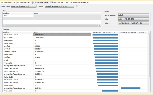
I can’t explain this problem, although I can speculate that it may have to do with the cramming of all the hidden nodes into a single layer. I can’t confirm that SSDM always uses a single hidden layer, but I saw no evidence that it built more than one in any of the models in this week’s trials. This was verified through the Generic Content Tree Viewer, which can be difficult to use even with simpler algorithms because of the complexity of SSDM’s metadata. As explained in past posts, the nine algorithms return results that can’t easily be compared, like apples and oranges; SSDM returns these results in a common format, however, which can be likened to a produce stand that sells both apples and oranges. The price to be paid for this convenience is that the columns in this common metadata format sometimes vary subtly in meaning not only from one algorithm to another, but also within each algorithm depending on the NODE_TYPE value. The Neural Network algorithm is especially complex in this respect because it had seven different node types, as depicted in Figure 14. As usual, we also have to deal with a second level of denormalization in the nested NODE_DISTRIBUTION table, in which the meaning of the standard columns ATTRIBUTE_NAME, ATTRIBUTE_VALUE, SUPPORT, PROBABILITY and VARIANCE changes from one row to the next depending on the VALUETYPE. At least this particular algorithm is limited to using VALUETYPE codes we’ve already encountered before, such as those indicating a Missing value, Discrete, Discretized or Continuous column, or a coefficient. The difficulty in interpreting the results is compounded further with this mining method, however, by the fact that we’re trying to represent a network in a tree structure. Moreover, the nodes are given numeric names as described in last week’s tutorial, which aren’t user-friendly. BOL also warns that “if more than 500 output neurons are generated by reviewing the set of predictable columns, Analysis Services generates a new network in the mining model to represent the additional output neurons,” but I have yet to encounter this scenario.
Figure 14: Metadata for the Neural Network Algorithm (adapted from Books Online as usual)
The ultimate difficulty with neural nets, however, is that no matter how your metadata is presented, it’s going to be next to impossible to track down exactly what a particular combination of weighted nodes represents. I won’t torture the readers with the screenshots, but basically the Generic Content Tree Viewer just shows you long lists of nodes with fractional ATTRIBUTE_VALUE numbers ranging between -1 and 1, which in turn refer to other nodes with the same incomprehensible decimal values. In other words, it’s just like trying to interpret a man’s thoughts from studying a slice of their cerebellum. You can certainly use the Generic Content Tree Viewer – or any other visualization of the inner workings of any neural net for that matter – to see how the network is constructed, which might be useful in repairing it. For example, you might be able to detect that a particular net is stuck in what’s termed a local minima because there aren’t enough nodes, or too many, or whatever. But you’ll never find the answers that SSDM returns hard-coded into a particular node; like human thoughts, they are not located in a single space, but pervade the entire network, like an electrical field effect. One of the brilliant aspects of the design of biological brains is how resistant they are to data loss, which is a benefit a DBA can certainly appreciate. Take away a dozen of the one hundred brain cells that contribute to the perception of the color turquoise or beige or whatever[xiii] and you may still perceive that particular color, albeit less strongly. The way the brain is designed makes it adept at encoding amounts of information so vast that our conscious minds ironically can’t conceive of it, yet at the same time this same scaffolding adds many layers of redundancy without any added expense. There is a trade-off though: the sheer complexity of it all means that it might be practically impossible to read a man’s thoughts in a mechanical or mathematically quantifiable way – which ought to make science fiction breathe a sigh of relief, given how often mind-reading is envisaged as a danger in dystopian futures. It might even be classified as an extra benefit of the design for that reason, but it is a definite drawback when we’re trying to create artificial neurons. We can make them encode functions in a way that is crudely analogous to a living brain, but we may never know exactly why they “think” what they do simply by dissecting them. As you can see, I was unable to do an autopsy on my neural nets to see why they were so unstable from one iteration to the net. This is a perfect example of why neural nets are a very poor choice when you need to understand explicitly how your data mining method dug up a particular result. It’s also why neural nets should never play anything more than an advisory role in mission-critical systems. When an airplane crashes, investigators can always retrieve the black box recorder. If it was a flown with the aid of a neural net, then the crash may have been caused by a black box of a different sort that can’t be interpreted at all.
This is an inherent limitation of the algorithm that future advances in mathematics and computing might not be able to solve, ever. I can think of a thousand different ways to enhance neural nets to make them more useful, particularly through modularization and allowing fine-grained customization. If users could substitute their own activation functions at certain nodes and specify certain topologies, particularly multidimensional ones, the range of problems that neural nets can solve would probably grow exponentially. In the future it might not be possible to plug Boltzmann machines into backprop nets, but it ought to be, because I have seen first-hand how surprisingly useful such combinations can be. The neural net I built a dozen years or so ago within minimal experience and investment of time had more than three dimensions, which is more than SSDM is capable of at the present. Hopefully in the future we will have tools capable of taking the grunt work out of building such structures. If so, we will need better visualization tools, such as animations of waves being fed forward or back propagated across a network of neurons, but it will be particularly difficult to visualize nets with more dimensions than the human eye can perceive. It’s easy to build them but quite difficult, if not physically impossible, to visualize them, which will compound the difficulty of interpreting the inner workings of neural nets further. Additional advances in biology may shed more light on how we can improve our artificial neural nets, or perhaps advances in the former will aid the latter in reverse, as was the case in the days of McCulloch and Pitts. I suspect that it will become standard practice to train many types of neural nets, especially those involving matrix math, in cubes and relational databases rather than in specialized math software, spreadsheets or middle tier objects, simply because these calculations can be performed faster r with set-based processing. The “Big Data” explosion will probably also make it prohibitively expensive in terms of resources and risks of data loss to process them anywhere else but in database servers. Server processing power is not the major determinant of how well a particular neural net functions, however, because the shape, topography and arrangement of functions within it determine its usefulness to a far greater extent. If neural nets do find more mainstream uses in the remainder of this century, they will probably have to be crafted by specialized net designers who can glue together the right combinations of constituent components to solve a particular problem. This is basically what I did when I tailored my first neural net to fit the particular problem topography presented by Go. As you can see from the erratic results I received from this week’s trials, I still have a lot to learn about designing them.
You can also probably tell that I am eager to learn about them. I am not half as enthused about Association Rules, the subject of the next installment of this series. We’ll basically be whip-sawing from my favorite algorithm to my least favorite, simply because Association Rules is the first of a set of three mining methods that group common items together. Association Rules is the subject of a lot of academic research today, but my guess is that we’re already reaching the top of the bell curve, after which future investments of resources will yield declining levels of improvement. The sky is still the limit with neural nets. The sharp contrast between the two may ultimately stem from the diametrically opposed ways in which they approach data mining. Neural nets are intricate and difficult to understand, but there are situations in which a method is called for that is easy to comprehend. Association Rules is a simple and popular data mining method, for the same reasons that a shovel is a simple and popular method of digging holes in the ground. There is a limit to how far you can dig with brute force methods like shovels, but sometimes they are the right tools for the job at hand.
Whenever I need a name for a new hard drive partition, I usually consult the Wikipedia webpage “List of Fictional Computers,” at http://en.wikipedia.org/wiki/List_of_fictional_computers
[ii] The 21st Century really could have mad scientists who are all too adept at misusing data mining methods like neural nets for all kind of nefarious purposes we haven’t even dreamt of yet, but they won’t be creating Frankenstein on a silicon wafer; they may think they have created life, but subjective reasoning – which the Turing Test is a supreme example of - is a mark of madness.
[iii] I played Go several times while in graduate school with a Chinese roommate, who really took me to school. He was a great guy, but the Taiwanese military trained him how to go without sleep, which didn’t mesh well with my insomniac personality.
[iv] Back then, I had a hard time even running SQL Server 6.5, which used to crash my machine routinely. I got my Microsoft Certified Solution Developer (MCSD) certification in Visual Basic 6 right about the time .Net came out, but my Compaq couldn’t handle the beta version without freezing up.
[v] Crivat, Bogdan, 2008, response to the post “BackPropagation Paper”at the MSDN Data Mining Forum, July 30, 2008. See http://social.msdn.microsoft.com/Forums/en-US/sqldatamining/thread/f2aeed0e-7002-4ec6-ba17-2acb430faa3f The book he cites is Bishop, Christopher M., 1996, Neural Networks for Pattern Recognition. Oxford University Press: U.S.
[vi] The figure 100 billion is widely cited but the IO9 webpage “The 4 Biggest Myths About the Human Brain” (available at http://io9.com/5890414/the-4-biggest-myths-about-the-human-brain) provides the more accurate, empirically tested figure of 86 billion. For the number of synapses, see the Wikipedia article “Neuron” at http://en.wikipedia.org/wiki/Neuron
[vii] A couple of starting points for this fascinating issue are the Wikipedia webpages “Quantum Mind” at http://en.wikipedia.org/wiki/Quantum_mind and “Quantum Brain Dynamics” at http://en.wikipedia.org/wiki/Quantum_brain_dynamics. The practice of citing Wikipedia on controversial issues is often knocked, but it can be a good first source to familiarize yourself with what a given issue is all about, regardless of how objective or biased the article’s content may be; it can be a first source as long as it is not the last source, so to speak.
[viii] McCulloch, Warren and Walter Pitts, Walter, 1943, “A Logical Calculus of the Ideas Immanent in Nervous Activity,” pp 115–133 in Bulletin of Mathematical Biophysics, Vol. 5. Like a lot of the other research papers I have cited in this series, I haven’t actually had the fortune of reading even the abstract, but I’ll provide the citation anyways in case anyone wants to follow up on the topic.
[ix] For the history of the algorithm, see Clabaugh, Caroline; Myszewski, Dave and Pang, Jimmy, 2000, “Neural Networks,” at the Stanford Univeristy Faculty website. “Created for Eric Roberts’ Sophomore College 2000 class entitled “The Intellectual Excitement of Computer Science” and available at http://www-cs-faculty.stanford.edu/~eroberts/courses/soco/projects/neural-networks/History/history1.html; Russell, Ingrid, “Brief History of Neural Networks,” reprinted at the Stanford University Faculty website. Available at http://uhaweb.hartford.edu/compsci/neural-networks-history.html. Also see the Wikipedia articles on “Back Propagation” at http://en.wikipedia.org/wiki/Backpropagation; “Delta Rule” at http://en.wikipedia.org/wiki/Delta_rule; “Feedforward Neural Network” at http://en.wikipedia.org/wiki/Feedforward_neural_network
[x] Reilly, Douglas; Cooper, Leon N.; and Elbaum, Charles, 1982, “A Neural Model for Category Learning,” p. 35 in Biological Cybernetics. Vol. 45, No. 1.
[xi] See the MSDN webpage “Microsoft Neural Network Algorithm Technical Reference” at http://msdn.microsoft.com/en-us/library/cc645901.aspx I must confess I was a bit confused by the terminology after reading some other explanations of these activation functions at other sites, which suggested that the sigmoid smoothing mechanism used in neural is also itself a form of hyperbolic tangent function.
[xii] See the Wikipedia article “Boltzmann Machine” at http://en.wikipedia.org/wiki/Boltzmann_machine
[xiii] Whatever they are. If you know what those colors are, you may find yourself the butt of an inside joke in a particular circle of friends I have, but all in good humor.


