Thankfully, the simplest of SQL Server’s algorithms is not quite as naïve about data mining as I am.

            As mentioned in my last post, I had to delay my article on the simplest of Microsoft’s data mining algorithms due to a number of factors, the worst of which turned out to be my own unfamiliarity with nested tables. This led to a lot of unforeseen performance problems that I have been able to work around for the time being by denormalizing the data source view (DSV) and schema mentioned in A Rickety Stairway to SQL Server Data Mining, Part 0.2: How to Dig Out of a Data Mining Cave-In. For an in-depth discussion of how the SQL Server IO data we will be mining for the rest of this series was collected and smoothed, refer to that post. For the time being, I will be using a simplified, denormalized version of the DSV in that post, which nonetheless produced some quite interesting and useful results with a minimal investment of training, time and energy when processed with Naïve Bayes, the most lightweight of the SQL Server Data Mining (SSDM) algorithms. Once the data collection phase was out of the way and the performance problem associated with my misuse of nested tables was avoided, it took only minutes for SSDM to return useful statistics that could help even a novice data miner and would-be DBA like myself to identify possible IO bottlenecks. This merely proves my original contention, that this vastly underrated and virtually unknown part of SQL Server can be put to really productive uses by people like myself, who have little background in statistics but some training in database administration. As I’ve said before, I’m not really qualified to write this tutorial series – but that’s the point.

           Many of the columns designated with a Content type of Continuous in the screenshot of that original DSV will be changed to Discretized for this week’s trial, because Naïve Bayes, allows only Key, Discrete and Discretized columns. For a refresher on the critical differences between Content types, see the first post in this series
A Rickety Stairway to SQL Server Data Mining, Part 0.0: An Introduction to an Introduction. Suffice it to say that we can include the Continuous columns by designating them as Discretized, but this means they are treated as independent states rather than as cumulative values; the millionth row in space_usedTable is ranked no higher than the first, for example. Keep in mind throughout today’s post that we may see ranges of values being compared, but Naïve Bayes is not aware that one range is higher than another; for example, the CpuTicks column has two ranges labeled 712016680402476-851112177387993 and 119571617179526-605322349738604, but SSDM will not take into account the fact that 851112177387993 is more than 605322349738604. They are merely treated as states of the objects that are thrown into buckets. I have left all of the parameters that can be used to refine the number of buckets, attributes states and the like at their default values for now; we will postpone playing with these variables for later in the series, but for a brief introduction to them, refer to my last post. I will use the Content types from my last post whenever possible in these trials, but in cases like Naïve Bayes, we have to substitute Discretized content designations for our Continuous and Cyclical columns whether we want to or not. This is an intrinsic limitation dictated by the internal math and logic of the algorithm itself. The whole point of Naïve Bayes, in fact, is to extract as much data as possible without the added complexity of taking the dependence of column values on each other into account. This enables it to make faster assessments of data than the other SSDM algorithms, but with results that are consequently less sophisticated. That is why it is often used for initials explorations of data, which makes it an ideal place to begin our foray into SSDM. What we discover here can then be used to ask the right questions when we apply more advanced algorithms.

The Brilliant Simplicity of Naïve Bayes

                Don’t let the name fool you; Naïve Bayes may be less sophisticated than the other algorithms, but it can still spit out results that are surprisingly useful. There are many variations on the algorithm and complex analyses of it in the academic literature, but the idea is actually quite simple at heart: instead of merely calculating the probability of an event, property or other state of an object, it takes existing evidence into account to adjust the conclusions (or “beliefs,” in Bayesian terminology) accordingly. This feedback mechanism is analogous to the scientific method, another useful tool that has quietly faded into desuetude in many branches of academia that call themselves sciences. It is basically a brute force method of computing probabilities, with some educated refinements based on prior knowledge – or as Books Online (BOL) puts it more elegantly, it “calculates the probability of every state of each input column, given each possible state of the predictable column” and “lists each input column in the dataset, and shows how the states of each column are distributed, given each state of the predictable column. You can use this view to identify the input columns that are important in differentiating between states of the predictable column.” This may help us decide which columns to set as inputs and predictables when using more sophisticated data mining algorithms. It is less brutish than mere probability and a little less forceful than merely doing a fancy Carsteian product of the input node probabilities – yet it is also quite unsophisticated compared to other algorithms, given that the values being analyzed are treated as unrelated states. For example, if you have four oranges in one basket and five in another, it will not be able to tell that there is one more in the second basket; four and five are simply states of the object, like names of people or GUIDs. Furthermore, the probability distributions of the two baskets are treated as independent of each other, so that if you had only five widgets to store in them, putting three in Basket A would not increase the chances of two widgets appearing in Basket B. This blindness – or conditional independence, to use a more politically correct term – is complemented by a related problem, the fact that it can only establish a relationship between two facts, without demonstrating whether the first caused the second or vice versa. These challenges were probably what fooled many scientists over two centuries into believing that Naïve Bayes was of little use. It was actually forgotten after its development by Thomas Bayes (1701–1761) and refinement by fellow mathematician Richard Price (1723-1791), then discarded once again after a colleague of greater reknown, Pierre Simon Laplace (1749-1827), rediscovered and refined it further. It did not become a popular tool until the invention of computers in the mid-20^th Century. Since then, it has become a useful instrument “in a range of fields including science, engineering, medicine, and law” as well as economics and game theory, and can be used for such tasks as classification, prediction, model selection for hypothesis testing (which make use of the Schwarz criterion and the likelihood function), sequences of events and searches, among other things.[ii] In SSAS, we are mainly concerned with Bayesian classification, although the results could probably be applied to any of these other purposes.

           The Microsoft variation of it is based on refinements introduced by D. Heckerman, D. Geiger, and D.M. Chickering in their 1995 research paper “Learning Bayesian Networks: The Combination of Knowledge and Statistical Data,” including two mathematical properties they call event equivalence and parameter modularity which are used to formulate better corrections.[iii] I may be the one in need of better corrections, but my understanding of the paper includes the idea that information loss can be minimized in Naïve Bayes by taking into account prior knowledge of additional relationships in data, such as the possibility that value A and value B may only be conditionally independent of each other when a third variable C is taken into account. There are many other variations on the algorithm out there in the wild world of machine learning research, many of which are associated with a low probability of comprehension without a Ph.D. in mathematics. I won’t get into a technical discussion of the nuances and differences between Bayes’ theorem, Bayes’ rule, the Bayes factor, Bayesian interpretation and Bayesian inference and the like for the highly practical reason that I don’t really understand them that well.[iv] That would obviate the point of this whole tutorial series, which aims to show that any competent DBA can glean useful information from SSDM, not to inspire people to get a doctorate in statistics, as appealing as that may be. We ought to at least be familiar with a few key terms, however, like prior distribution, or the distribution of data expected before any observation takes place; the sampling distribution or likelihood, which represents the data distribution after observation; the marginal likelihood or “evidence,” which is the distribution after the data has been marginalized out[v] and the posterior distribution, or the data distribution output by the algorithm.[vi] To make a long story short, you calculate the expected distribution of data, make an observation of it, whittle it down and then the algorithm coughs a posterior distribution back out at you. Many researchers have tried to pinpoint why Naïve Bayes spits back useful posterior distributions so often despite the manifest blindness of its inputs and have reached a variety of conclusions, all of which may be true. On theory is that it depends on a zero-one loss function for correction rather than the more well-known statistical method of squaring the errors, which allows records to be accurately classified even when the probability is misjudged.[vii] Another is that Naïve Bayes is most effective when the actual independence of the values from each other are either highly dependent or completely independent of each other.[viii] It is a bit like the German proverb against “sitting between two stools.”[ix] If the latter explanation is true, it may signify that data with little variation (i.e., it has “low entropy” because it follows a uniform distribution curve) or relatively high variation may be good candidates for Bayesian examination. We can calculate the distribution of our data fairly efficiently on the relational side using built-in T-SQL functions for standard deviation and the like, or through the new analytic windowing functions. This may later come in handy when judging how reliable the results returned by our data mining model may be in the future, so that we can make better choices on which to use as inputs and predictables in more computationally expensive data mining methods.

Visualizing the Results

                One of the best aspects of SSDM is that it provides several means of visualization right out of the box, which require no programming on the data miner’s part. Simply create your mining model and process it as directed in the last few posts, then several easily interpretable graphs will become instantly available on the Mining Model Viewer tab in SQL Server Data Tools (SSDT). Here’s tip to keep in mind: a dialog box may prompt you to reprocess the model whenever you select that tab, but quite often the model content will not actually be out of date, so be aware of that. Make sure you have the right model selected in that tab’s Mining Model dropdown box (long ago, I selected the wrong model and was left baffled by the results I received, so keep an eye out for that) and then select the appropriate visualization method in the Viewer dropdown. Microsoft supplied eight types of viewers but your choice of algorithm will limit the ones available. In this case, we are limited to the Microsoft Naïve Bayes Viewer and the Generic Content Tree Viewer, the latter of which provides a rawer view of the data that the first uses to produce its fancy graphs.

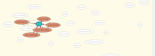
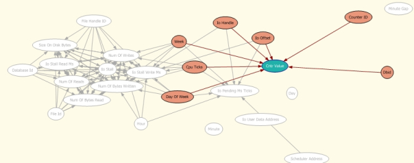
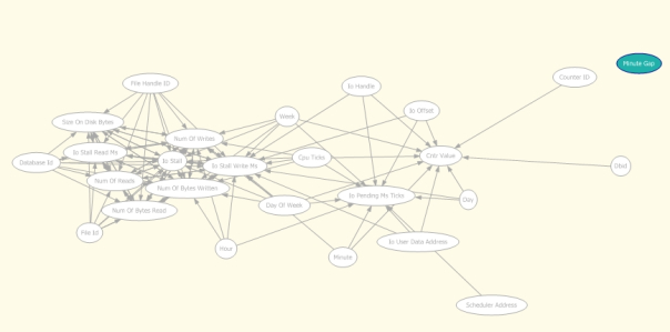
               The Mining Model Viewer tab has four tabs of its own when the Naïve Bayes Viewer is selected, the first of which is the Dependency Network. This displays a complex network of relationships between the input and output attributes, as depicted in Figure 1. By dragging the All Links slider down we can eliminate less likely relationships, thereby allowing us to focus on more important ones. We can also highlight the relationships relevant to a particular oval by clicking on it, as depicted in Figures 2 through 4, in which the selected attribute in in blue, the attributes that predict it are in orange and those that predict both way are depicted in purple. In this week’s trial, we are comparing a single denormalized view representing the relationships between the dm_io_pending_io_requests, dm_io_virtual_file_stats and dm_os_performance_counters tables we created during our data collection process (all of which were linked to a parent RecordTable prior to denormalization), as discussed in the last post. Not surprisingly, the links between the tables that the view references are not as common or strong as those between the particular columns within each. By sliding the All Links tab and selecting the oval for the dm_os_performance_counters column cntr_value,  however, we can see that it does have a moderately strong tie of some kind to IOHandle and IOOffset from dm_io_virtual_file_stats, as seen in Figure 3. Those two columns, along with several others, were also tied to the important IOPendingMsTicks column from dm_io_pending_io_requests, which is not depicted below for brevity’s sake. The strongest relationships between any of the columns were for those related to IOStall, which is one of the critical measures we’d like to keep an eye on, since it might help us identify any bottlenecks in the IO subsystem. As I mentioned in the last post, I had to create a special measure called MinuteGap in the RecordTable to deal with gaps between the SQL Server Integration Services (SSIS) jobs that were supposed to occur every minute during the data collection process. Perhaps at some point in this series our data will shed some light on that mystery, but from the lack of relationships depicted in Figure 4, we’re still in the dark for now.

Figure 1:The Dependency Network Tab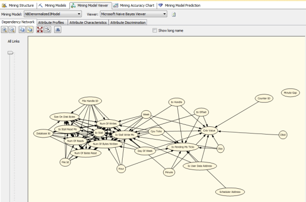

Figure 2: IOStall

Figure 3: CntrValue

Figure 4: MinuteGap

                SSDT has some great visualization tools that you can use right out of the box with little prior experience, but my least favorite has to be the Attribute Profiles tab. By selecting one of your model’s predictable attributes in the Predictable dropdown box, you can bring up a diagram like the one in Figure 5; each row represents a particular input attribute and each column header refers to a specific bucket of values for the predictable output attribute we’ve selected. Think of it as a table, except that each cell is populated with a histogram instead of a single value as we’re accustomed to seeing in the relational database world. The number of  histogram bars can also be adjusted through a drop-down box. The histograms are useful once you know how to interpret them, but the variety of colors used to depict the distinctive values for each state make it all difficult to decipher at first glance. It might be easier to interpret if the color were shaded by gradations in tandem with the values, but this wouldn’t be possible at all with algorithms like Naïve Bayes that can only use Discrete or Discretized columns; the algorithm itself has no knowledge that these ranges indicate any rank or order. Keep in mind that all of the states you see below are discrete or discretized values, which means that they are treated as having no relationship to each other, like the values M and F might in a gender column in a relational database. By clicking on a particular histogram or hovering over one, we can view the probability distributions for all of the buckets for that input attribute, when compared against that particular bucket for the the predictable attribute we’ve chosen to look at. In the example below, the Mining Legend and balloon seem cluttered with undecipherable nonsense, but those long numbers on the left are merely the names assigned to the CpuTicks buckets, which represent really high numeric ranges. When a less cluttered column is selected, the results are a lot easier to read, so that we can easily retrieve the probability distributions at a glance. Once you become familiar with SSDM, it becomes easier to tune out the necessary clutter that these long numeric names represent, which are more of a problem when using the Generic Content Tree Viewer or retrieving the values with MDX queries.

Figure 5: The Attribute Profiles Tab}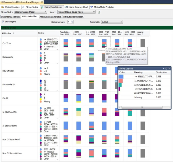

           In the graphics above we were examining IOStall again, since we now know that it has some strong relationships with other columns. In Figures 6 and 7 we’re looking at high values for NumOfWrites and NumofReadss, since we already know that they strongly predict IOStall and would understand our IO bottlenecks better if we know what caused those high read and write numbers in turn. The Attribute Characteristics tab is easier to understand that Attribute Profiles, in part because it allows us to limit our view to a single bucket or state for a predictable attribute, thereby reducing the kind of information glut that can occur with the maze of histograms above. Simply use the Value dropdown to select a state or bucket from the column you chose from the Attribute dropdown and a graphic like the one below will appear. It’s all fairly straightforward; the longer the blue line is, the higher the probability that the input state on the left will be associated with the particular state of the single predictable attribute we’ve chosen. You can sort the results by clicking on the column headers labeled Attributes and Probability. Perhaps the only confusing aspect of this for a novice might be that the same attribute names may be listed more than once on the left. That is because each attribute has more than one state or bucket associated with it, some of which may also have high enough probabilities of being associated with our output state to warrant inclusion. Each pair attribute-value pair is therefore unique, not each attribute.

Figure 6: Attribute Characteristics for a NumOfWrites Bucket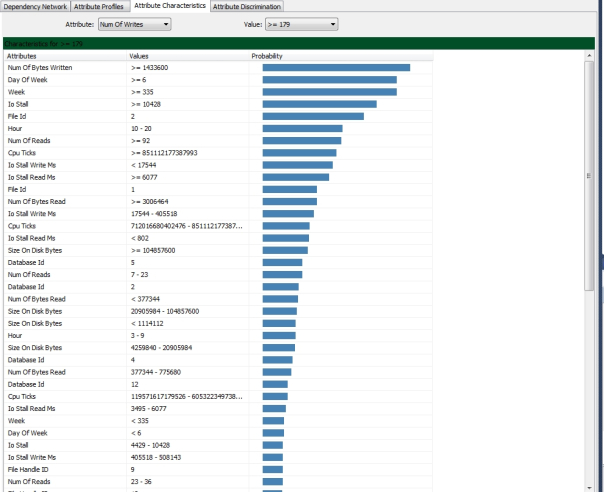

Figure 7: Attribute Characteristics for a NumOfReads Bucket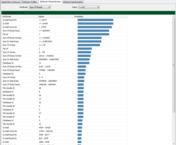

           The Attribute Discrimination tab is a little more complex but can yield some really valuable information. On this tab we’re comparing an input state or bucket against two states of the single predictable output attribute we’ve selected, rather than just one. If the blue bar appears on the left, the probability favors the output state in the Value 1 dropdown boxand if it’s on the right, it favors the one selected in the Value 2 dropdown. As in the Attribute Characteristics tab, the longer the bar, the greater the probability. It is also possible to test a particular bucket against all others by selecting the value “All other states” from one of the two dropdowns. What Figure 8 tells us is that there is a relatively high probability that FileID #1 will be associated with 1 to 5 writes, while FileID #2 is associated with very high write activity of greater than or equal to 179. Relatively high values for IOStall and NumOfBytesWritten are strongly associated with a high number of Writes, while lower values for NumOfBytesWritten strongly favor very low values for NumOfWrites. None of this is unexpected, given that most consumer hard drives don’t write as fast as they read, thereby causing stalls. That does confirm, however, that the Naïve Bayes algorithm is finding some of the relationships that it ought to, despite the fact that a fairly small dataset is being fed into the simplest of Microsoft’s nine algorithms. This ought to boost our confidence in its capabilities, so that when it discovers potentially useful but previous unknown relationships – such as the well-defined patterns for write activity on those two particular database files – we can trust it enough to feed the results into a more complex and resource-intensive algorithm.

Figure 8: Attribute Discrimination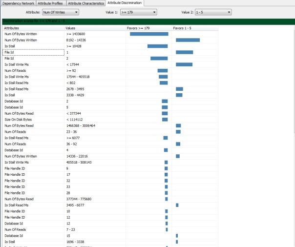

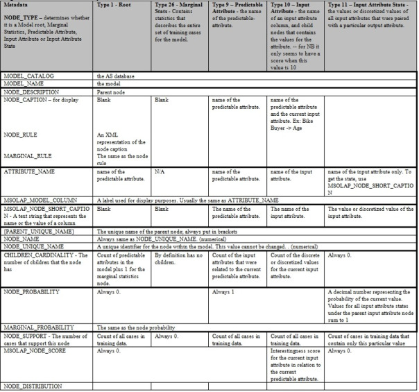
                Stouthearted statististical spelunkers may want to dig deeper into the data that these visualization methods make use of. Once our survey of the nine algorithms is finished, I hope to write in-depth about how to write DMX queries, which the most fundamental means of getting to the bottom of the mine, so to speak. For now, however, we will stick with the simpler method of using the Generic Content Tree Viewer, which can be selected in the Viewer dropdown no matter what algorithm is being used. Interpreting this extra detail will be difficult, however, without some understanding of SSDM’s common metadata format. The nine algorithms return data that is sometimes intrinsically more difficult to compare than apples and oranges, so it is remarkable that Microsoft’s data mining team was able to devise a format that can hold both apples and oranges simultaneously. I discuss that format in more detail in A Rickety Stairway to SQL Server Data Mining, Part 0.1: Data In, Data Out, but as a quick refresher, keep in mind that there are five possible NODE_TYPE values with Naïve Bayes: 1 for the root node; 9 signifies a predictable attribute; 10 refers to an input attribute and its children; 11 is for input attribute values paired with output value attributes; and 26 is for a Marginal Stats node, which provides information on the training cases. Several of these nodes may have child nodes, which may be crammed together if a DMX query is written so that it returns denormalized results; one of the advantages of the Generic Content Tree Viewer is that it returns the same information, but without the data miner having to write complex DMX code to return it in a tree structure. The most important columns with Naïve Bayes are in the NODE_DISTRIBUTION table, which is also nested and has the same columns as when we’re using other algorithms: NODE_CAPTION, ATTRIBUTE_NAME, ATTRIBUTE_VALUE, SUPPORT, PROBABILITY and VALUE_TYPE It will be empty, however, unless we’re dealing with a NODE_TYPE value 11 (input attribute value pair) or 24 (Marginal Stats).

          A couple of posts ago, I went into more detail about how the common format for SSDM results may vary from algorithm to algorithm. Figure 9 shows how the format differs specifically with Naïve Bayes.  Some of these columns, such as NODE_PROBABILITY, MARGINAL_PROBABILITY, MS_OLAP_NODE_SCORE, MSOLAP_MODEL_COLUMN and MSOLAP_NODE_SHORT_CAPTION are of no consequence to us with Naïve Bayes, while others like ATTRIBUTE_NAME, MODEL_CATALOG and MODEL_NAME are just object identifiers for the column, database and mining model respectively. CHILDREN_CARDINALITY simply tells us how many child nodes a particular node has, while the NODE_SUPPORT is simply the number of cases taken into account for that node.

Figure 9. Metadata for Naïve Bayes (adapted from Books Online)

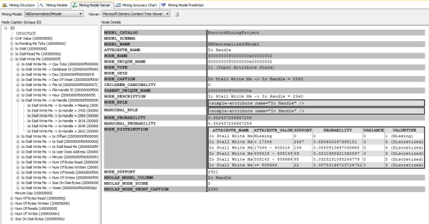
                Once we have a minimal understanding of what these result columns signify when we’re dealing with Naïve Bayes, we can use the Generic Content Tree Viewer to return the statistics for a specific node, such as the probability distributions and case support numbers. In Figure 10, we can see that each of our predictable attributes has its own node under the root node. If we drill down another level, we see each predictable output compared against the relevant input attributes; drilling down another level below that takes us to the lowest leaf nodes, in which our output is compared against a particular input state and NODE_DISTRIBUTION statistics are made available. A leaf node comparing six different buckets of IOStallWriteMs values against a single state of the IOHandle input attribute is shown in the graphic below. The two main obstacles to interpreting the results of the Generic Content Tree Viewer are the differences between the meanings of the columns depending on the algorithm, as well as the long numbers next to each node, which are merely autogenerated numeric names rather than important statistics. Just keep in mind that their only purpose is identification, not to add information to the model.

Figure 10 – An Interesting Type 11 Node in the Generic Content Tree Viewer – Click to Enlarge

                The Generic Content Tree Viewer also provided really useful information at a casual glance about three FileHandleIDs which had unusually high values for IOStall, at least in comparison to the other 37 nodes comparing IOStallWriteMs states against FileHandleID values. For the sake of brevity I’m not including screenshots, but FileHandleID #9 had an 80.5 percent probability of being associated with IOStallWriteMs values between 17544 and  405518, while #12 had a 65.8 percent chance and  #17 had a 21.1 percent chance. All of these values were high in comparison to the 34 FileHandleIDs, while the latter two also had high values for three buckets of even greater values for IOStallWriteMS. A few minutes of looking at the Generic Content Viewer and the Attribute Discrimination tab thus turned up valuable information about specific files with unusual write activity that could be causing bottlenecks. Because Naïve Bayes already confirmed some obvious relationships we expected to find, such as the close ties between IOStall and high read and write activity, we know that its results can be trusted to return good data at least part of the time. There are certainly many simpler tools out there that can help a SQL Server DBA identify a particular file that might be causing bottlenecks, but SSDM can be used to build solutions much more sophisticated than that. I don’t have the expertise to do that; I wanted to kill two birds with one stone by learning more about IO while simultaneously referring to subject matter that experienced DBAs already have some familiarity with. It provides us with a proof-of-concept that SSDM could potentially be used to give us a more sophisticated analysis of performance bottlenecks, which is just one of a dizzying array of constructive uses it could be put to. The workflow for more sophisticated data mining projects often begins with Naïve Bayes, which is merely the beginning of what can be done with SSDM. In A Rickety Stairway to SQL Server Data Mining, Algorithm 2: Linear Regression we will see what happens when we take the inputs and outputs Naïve Bayes has identified here, then feed them into a slightly more resource-intensive algorithm that allows Continuous columns.

For this account of the history of the algorithm, see the Wikipedia page “Bayes’ Theorem.”