Introduction

Having seen a number of Microsoft Business Intelligence implementations, I have noticed that surprisingly few use precalculated closing balances and semi-additive measures in SQL Server. I think this may be partly because of a lack of good examples available, and therefore decided to write about this issue.

This article is mainly divided in the following sections:

1. Background describing a simple example of closing balances
2. Description of our example data - a Balance Sheet
3. Step by step how to precalculate closing balances and build a cube for our Balance Sheet
4. Test results and conclusion

Background

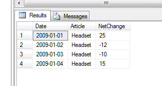
The Inventory problem is a typical example of a semi-additive measure. Imagine that you have an ERP-system that tracks inventory, recording every time an item is in- or out of the inventory. From the ERP-system you get a daily net-change for each item as shown below:

However, what the management is interested in is not the net changes, but the quantity available at the end of every day:

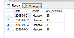
When looking at a specific day, month or other period, the quantity available is the sum of all net changes from beginning of time to the end of the specific period. This is a closing balance.

The definition of a semi-additive measure is that it behaves differently in different dimensions. A closing balance is semi-additive because it behaves differently in the time-dimension than other dimensions. Other examples of semi-additive measures are: opening balance, average and by account.

Step by Step example - a Balance Sheet

Another situation, apart from inventories, where you want to work with opening and closing balances is Balance Sheets. When extracting general ledger data from an ERP-system you will get the net transactions. However, financial people are used to seeing opening balances, net changes and closing balances. This example will show how to produce closing balances, although opening balances can be produced very easily by small modifications to this example.

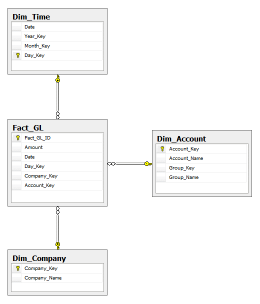
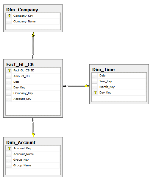
Consider the following star-schema for describing the Balance Sheet:

The fact-table is filled with transactional data (not necessarily in time-order):

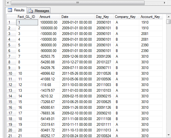
The Day_Key is expressed in ISO-format (YYYYMMDD), and the Month_Key and Year_Key are made up by simply removing lower parts:

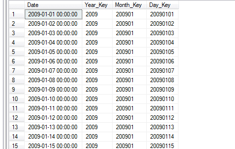
Dim_Account is a very simplified chart of accounts (based on EU-standards):

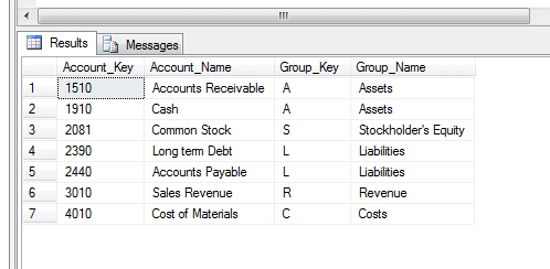
Natural keys are used in the relation between Fact_GL and the dimension tables in this example, whereas in a real-world solution surrogate keys should be used instead.

Precalculating the closing balances through T-SQL

Calculating the closing balances can be done in two ways: calculating them in dynamically in the OLAP Cube, or precalculating them in the relational database. We will try both in this example.

To precalculate the closing balances in the relational database, we create a new table to hold the calculated values, Fact_GL_CB, the is similar to the previous fact-table but contains field Amount_CB instead of Amount and also has an extra Date-file (not really necessary, but simplifies a bit):

We now need to fill Fact_GL_CB with closing balances. It should have a value for every combination of Company, Account and Day_Key, that is the sum of all amounts having a date less than or equal to the Day_Key. This can be accomplished using while-loops, cursors, etc. However I prefer writing a recursive SQL-query instead. My solution is in a few steps:

Initialise a range-table, telling the recursive query which dates to handle:

TRUNCATE TABLE Fact_GL_CB;

SELECT DISTINCT
 Company_Key,
 Account_Key,
 (SELECT MIN([Date]) FROM Fact_GL) AS [Date],
 (SELECT MAX([Date]) FROM Fact_GL) AS [MaxDate]
INTO #Range
FROM Fact_GL
WHERE Account_Key < N'3';

Note that this step also deletes any previous data from Fact_GL_CB and filters out transactions not belonging to the Balance Sheet (having Account_Key starting with 3 or higher). Using the name #Range ensures it is written to tempdb instead of PRECALCDB.

Next step is to create a daily sums table, holding the sum of all transactions each day:

WITH
AllDays AS
(
 SELECT 
 Company_Key, 
 Account_Key, 
 [Date], 
 [MaxDate]
 FROM #Range

 UNION ALL

 SELECT
 Company_Key, 
 Account_Key, 
 DATEADD(DAY, 1, [Date]), 
 [MaxDate]
 FROM AllDays
 WHERE [Date] < [MaxDate]
)
SELECT
 AllDays.Company_Key, 
 AllDays.Account_Key, 
 AllDays.[Date], 
 ISNULL(SUM(Amount), 0) [Amount]
INTO #DailySums
FROM AllDays
LEFT JOIN Fact_GL ON AllDays.Company_Key = Fact_GL.Company_Key AND AllDays.Account_Key = Fact_GL.Account_Key AND AllDays.[Date] = Fact_GL.[Date] 
GROUP BY AllDays.Company_Key, AllDays.Account_Key, AllDays.[Date]
OPTION (MAXRECURSION 0);

Note the option MAXRECURSION which is necessary to prevent the AllDays common table expression to hit the default recursion depth limit.

Having calculated the daily sums, the closing balances can be calculated using a recursive query that accumulates daily sums:

WITH
Accumulator AS
(
 SELECT 
 Company_Key, 
 Account_Key, 
 [Date], 
 [Amount]
 FROM #DailySums
 WHERE [Date] = (SELECT MIN([Date]) FROM #Range)

 UNION ALL

 SELECT
 #DailySums.Company_Key, 
 #DailySums.Account_Key, 
 #DailySums.[Date], 
 #DailySums.[Amount] + Accumulator.[Amount]
 FROM #DailySums
 JOIN Accumulator
 ON
 Accumulator.Company_Key = #DailySums.Company_Key AND
 Accumulator.Account_Key = #DailySums.Account_Key AND
 DATEADD(DAY, 1, Accumulator.[Date]) = #DailySums.[Date]
)
INSERT INTO Fact_GL_CB(Amount_CB, [Date], Day_Key, Company_Key, Account_Key)
SELECT
 [Amount],
 [Date],
 CONVERT(INT, CONVERT(NVARCHAR, [Date], 112)) [Day_Key],
 Company_Key,
 Account_Key
FROM Accumulator
ORDER BY Company_Key, Account_Key, [Date]
OPTION (MAXRECURSION 0);

Finally, the performance can be improved by adding an index on #DailySums between step 2 and 3.

Building the cube

Now we are finished with the relational database part and continue with the cube. We start an Analysis Services project in BIDS and create a Data Source View as below:

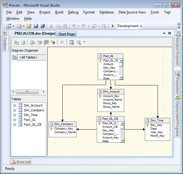
The next step is to create a cube and dimensions. This is most easily done by running the New Cube wizard. Make sure you select both Fact_GL and Fact_GL_CB as measure group tables. Select the dimensions. Be ready to make some adjustments to the dimensions (the wizard isn't too clever).

We also need to do minor adjustments to the measures. Change the format so that they are displayed as Currency or similar. Rename "Amount CB" to "Amount CB Precalc" and change the aggregation function to LastNonEmpty:

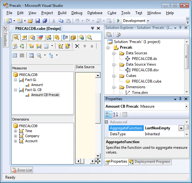
LastNonEmpty is basically the equivalent of a closing balance. Another option would be to use LastChild, which differs only in the handling of missing values.

Also we add a calculated measure, "Amount CB Cube", which dynamically calculates the closing balance in the cube (no need for any Fact_GL_CB table). This measure can easily be created as follows:

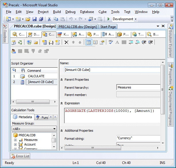
Build and deploy the solution. Now it's time to test it!

Results

To evaluate the results, I have used MDX Studio by Mosha Pasumansky. This is an essential tool that any serious Microsoft OLAP-developer should have.

The following MDX-query can be used to test. Swap [Amount CB Cube] for [Amount CB Precalc] to test the precalculated values instead of the dynamic values.

SELECT 
 {Account.Assets.CHILDREN, Account.Liabilities.CHILDREN} * 
 {[Amount], [Amount CB Cube]} ON COLUMNS,
 [Time].Day.MEMBERS ON ROWS
FROM PRECALCDB

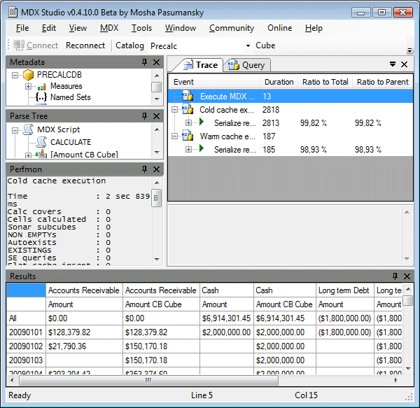
Using MDX Studio to profile this query gives us the following performance for dynamically calculated closing balances:

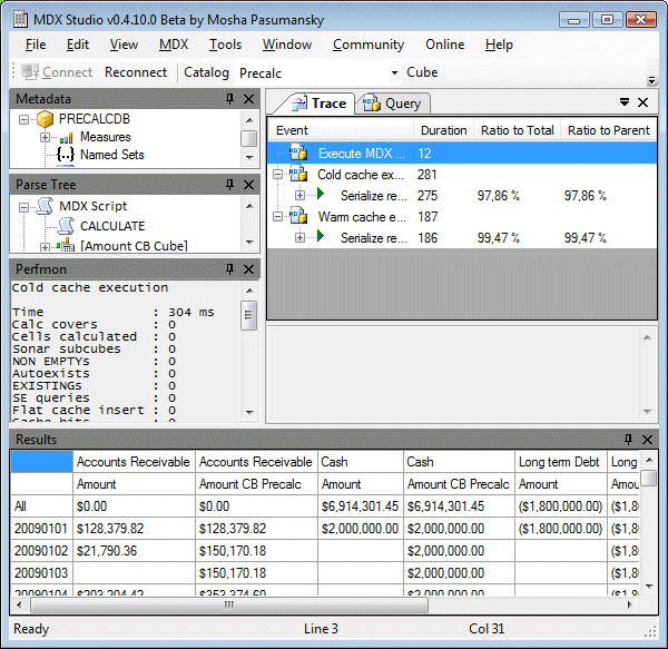
Testing the precalculated closing balances yields this performance:

Conclusion

As you can see, the precalculated closing balances are about 10 times faster when not cached. When cached the performance difference is insignificant, as could be expected since there is no need then to do any calculations.

However, the performance is not the only reason for using precalculations. It may not even be the most important reason. Calculating the closing balance dynamically in the cube (using a calculated measure) has several disadvantages, for example:

• Drill-through actions will not work
• Problems may arise with solve-order
• Calculated measures lack options such as Display Folder

Therefore the use of the precalculated semi-additive measures is much preferred when possible. Especially in the case that you already have closing balances or opening balances from the data source.