This article will show you how to calculate moving averages with Financial Market data across time using T-SQL. There are two moving averages used with technical analysis in the Financial Markets - Simple and Exponential. The goal here is to provide you with a solution that will allow you to do Simple Moving Averages (SMA) efficiently, and build upon that to do EMA's.
Simple Moving Average (SMA)
The difference between the normal average we use (i.e. via the AVG() function), and a simple moving average is that moving averages only use a subset of the whole data relative to the date in the current row. For example, in the stock market, many of the finance sites and charting tools feature a 20 day SMA (simple moving average) overlay on top of the stock price. The picture below shows the stock price of Google in dark blue, and it's 20-day SMA in light blue.
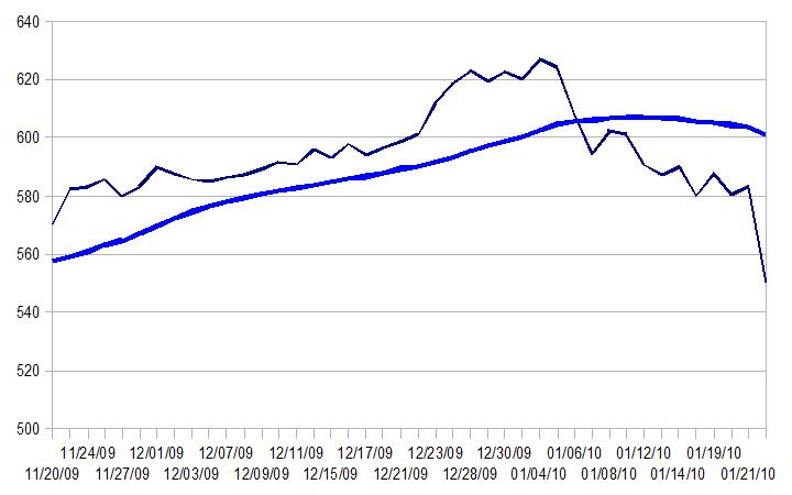
The data point at 12/30/09 for the 20 day SMA is at about $600. This average only includes the previous 20 trading days. As you can see it is a useful too for figuring out general trending patterns without being susceptible to short term volatility. However it's downfall is that it's a lagging indicator, and therefore isn't a good indicator of what the immediate future might hold. Regardless, this metric can be useful with any historical datasets for summary trending graphs and snapshots, whether it's for stocks, monthly income, or power consumption.
Implementation
At this point, I'm guessing most readers of this article already have the gears churning on how to solve this problem. So let's go through and entertain some strategies on how to accomplish this. Here is the setup code for this article which includes a our historical stock data for Google:
--Create our historical data table
create table #google_stock
(
quote_date [datetime],
open_price [decimal](6,2),
close_price [decimal](6,2),
high_price [decimal](6,2),
low_price [decimal](6,2)
)

INSERT INTO #google_stock (quote_date, open_price, close_price, high_price, low_price) VALUES ('20091026', 555.75, 554.21, 561.64, 550.89)
INSERT INTO #google_stock (quote_date, open_price, close_price, high_price, low_price) VALUES ('20091027', 550.97, 548.29, 554.56, 544.16)
INSERT INTO #google_stock (quote_date, open_price, close_price, high_price, low_price) VALUES ('20091028', 547.87, 540.30, 550.00, 538.25)
INSERT INTO #google_stock (quote_date, open_price, close_price, high_price, low_price) VALUES ('20091029', 543.01, 551.05, 551.83, 541.00)
INSERT INTO #google_stock (quote_date, open_price, close_price, high_price, low_price) VALUES ('20091030', 550.00, 536.12, 550.17, 534.24)
INSERT INTO #google_stock (quote_date, open_price, close_price, high_price, low_price) VALUES ('20091102', 537.08, 533.99, 539.46, 528.24)
INSERT INTO #google_stock (quote_date, open_price, close_price, high_price, low_price) VALUES ('20091103', 530.01, 537.29, 537.50, 528.30)
INSERT INTO #google_stock (quote_date, open_price, close_price, high_price, low_price) VALUES ('20091104', 540.80, 540.33, 545.50, 536.42)
INSERT INTO #google_stock (quote_date, open_price, close_price, high_price, low_price) VALUES ('20091105', 543.49, 548.65, 549.77, 542.66)
INSERT INTO #google_stock (quote_date, open_price, close_price, high_price, low_price) VALUES ('20091106', 547.72, 551.10, 551.78, 545.50)
INSERT INTO #google_stock (quote_date, open_price, close_price, high_price, low_price) VALUES ('20091109', 555.45, 562.51, 562.58, 554.23)
INSERT INTO #google_stock (quote_date, open_price, close_price, high_price, low_price) VALUES ('20091110', 562.73, 566.76, 568.78, 562.00)
INSERT INTO #google_stock (quote_date, open_price, close_price, high_price, low_price) VALUES ('20091111', 570.48, 570.56, 573.50, 565.86)
INSERT INTO #google_stock (quote_date, open_price, close_price, high_price, low_price) VALUES ('20091112', 569.56, 567.85, 572.90, 565.50)
INSERT INTO #google_stock (quote_date, open_price, close_price, high_price, low_price) VALUES ('20091113', 569.29, 572.05, 572.51, 566.61)
INSERT INTO #google_stock (quote_date, open_price, close_price, high_price, low_price) VALUES ('20091116', 575.00, 576.28, 576.99, 572.78)
INSERT INTO #google_stock (quote_date, open_price, close_price, high_price, low_price) VALUES ('20091117', 574.87, 577.49, 577.50, 573.72)
INSERT INTO #google_stock (quote_date, open_price, close_price, high_price, low_price) VALUES ('20091118', 576.65, 576.65, 578.78, 572.07)
INSERT INTO #google_stock (quote_date, open_price, close_price, high_price, low_price) VALUES ('20091119', 573.77, 572.99, 574.00, 570.00)
INSERT INTO #google_stock (quote_date, open_price, close_price, high_price, low_price) VALUES ('20091120', 569.50, 569.96, 571.60, 569.40)
INSERT INTO #google_stock (quote_date, open_price, close_price, high_price, low_price) VALUES ('20091123', 576.49, 582.35, 586.60, 575.86)
INSERT INTO #google_stock (quote_date, open_price, close_price, high_price, low_price) VALUES ('20091124', 582.52, 583.09, 584.29, 576.54)
INSERT INTO #google_stock (quote_date, open_price, close_price, high_price, low_price) VALUES ('20091125', 586.41, 585.74, 587.06, 582.69)
INSERT INTO #google_stock (quote_date, open_price, close_price, high_price, low_price) VALUES ('20091127', 572.00, 579.76, 582.46, 570.97)
INSERT INTO #google_stock (quote_date, open_price, close_price, high_price, low_price) VALUES ('20091130', 580.63, 583.00, 583.67, 577.11)
INSERT INTO #google_stock (quote_date, open_price, close_price, high_price, low_price) VALUES ('20091201', 588.13, 589.87, 591.22, 583.00)
INSERT INTO #google_stock (quote_date, open_price, close_price, high_price, low_price) VALUES ('20091202', 591.00, 587.51, 593.01, 586.22)
INSERT INTO #google_stock (quote_date, open_price, close_price, high_price, low_price) VALUES ('20091203', 589.04, 585.74, 591.45, 585.00)
INSERT INTO #google_stock (quote_date, open_price, close_price, high_price, low_price) VALUES ('20091204', 593.02, 585.01, 594.83, 579.18)
INSERT INTO #google_stock (quote_date, open_price, close_price, high_price, low_price) VALUES ('20091207', 584.21, 586.25, 588.69, 581.00)
INSERT INTO #google_stock (quote_date, open_price, close_price, high_price, low_price) VALUES ('20091208', 583.50, 587.05, 590.66, 582.00)
INSERT INTO #google_stock (quote_date, open_price, close_price, high_price, low_price) VALUES ('20091209', 587.50, 589.02, 589.33, 583.58)
INSERT INTO #google_stock (quote_date, open_price, close_price, high_price, low_price) VALUES ('20091210', 590.44, 591.50, 594.71, 590.41)
INSERT INTO #google_stock (quote_date, open_price, close_price, high_price, low_price) VALUES ('20091211', 594.68, 590.51, 594.75, 587.73)
INSERT INTO #google_stock (quote_date, open_price, close_price, high_price, low_price) VALUES ('20091214', 595.35, 595.73, 597.31, 592.61)
INSERT INTO #google_stock (quote_date, open_price, close_price, high_price, low_price) VALUES ('20091215', 593.30, 593.14, 596.38, 590.99)
INSERT INTO #google_stock (quote_date, open_price, close_price, high_price, low_price) VALUES ('20091216', 598.60, 597.76, 600.37, 596.64)
INSERT INTO #google_stock (quote_date, open_price, close_price, high_price, low_price) VALUES ('20091217', 596.44, 593.94, 597.64, 593.76)
INSERT INTO #google_stock (quote_date, open_price, close_price, high_price, low_price) VALUES ('20091218', 596.03, 596.42, 598.93, 595.00)
INSERT INTO #google_stock (quote_date, open_price, close_price, high_price, low_price) VALUES ('20091221', 597.61, 598.68, 599.84, 595.67)
INSERT INTO #google_stock (quote_date, open_price, close_price, high_price, low_price) VALUES ('20091222', 601.34, 601.12, 601.50, 598.85)
INSERT INTO #google_stock (quote_date, open_price, close_price, high_price, low_price) VALUES ('20091223', 603.50, 611.68, 612.87, 602.85)
INSERT INTO #google_stock (quote_date, open_price, close_price, high_price, low_price) VALUES ('20091224', 612.93, 618.48, 619.52, 612.27)
INSERT INTO #google_stock (quote_date, open_price, close_price, high_price, low_price) VALUES ('20091228', 621.66, 622.87, 625.99, 618.48)
INSERT INTO #google_stock (quote_date, open_price, close_price, high_price, low_price) VALUES ('20091229', 624.74, 619.40, 624.84, 618.29)
INSERT INTO #google_stock (quote_date, open_price, close_price, high_price, low_price) VALUES ('20091230', 618.50, 622.73, 622.73, 618.01)
INSERT INTO #google_stock (quote_date, open_price, close_price, high_price, low_price) VALUES ('20091231', 624.75, 619.98, 625.40, 619.98)
INSERT INTO #google_stock (quote_date, open_price, close_price, high_price, low_price) VALUES ('20100104', 626.95, 626.75, 629.51, 624.24)
INSERT INTO #google_stock (quote_date, open_price, close_price, high_price, low_price) VALUES ('20100105', 627.18, 623.99, 627.84, 621.54)
INSERT INTO #google_stock (quote_date, open_price, close_price, high_price, low_price) VALUES ('20100106', 625.86, 608.26, 625.86, 606.36)
INSERT INTO #google_stock (quote_date, open_price, close_price, high_price, low_price) VALUES ('20100107', 609.40, 594.10, 610.00, 592.65)
INSERT INTO #google_stock (quote_date, open_price, close_price, high_price, low_price) VALUES ('20100108', 592.00, 602.02, 603.25, 589.11)
INSERT INTO #google_stock (quote_date, open_price, close_price, high_price, low_price) VALUES ('20100111', 604.46, 601.11, 604.46, 594.04)
INSERT INTO #google_stock (quote_date, open_price, close_price, high_price, low_price) VALUES ('20100112', 597.65, 590.48, 598.16, 588.00)
INSERT INTO #google_stock (quote_date, open_price, close_price, high_price, low_price) VALUES ('20100113', 576.49, 587.09, 588.38, 573.90)
INSERT INTO #google_stock (quote_date, open_price, close_price, high_price, low_price) VALUES ('20100114', 583.90, 589.85, 594.20, 582.81)
INSERT INTO #google_stock (quote_date, open_price, close_price, high_price, low_price) VALUES ('20100115', 593.34, 580.00, 593.56, 578.04)
INSERT INTO #google_stock (quote_date, open_price, close_price, high_price, low_price) VALUES ('20100119', 581.20, 587.62, 590.42, 576.29)
INSERT INTO #google_stock (quote_date, open_price, close_price, high_price, low_price) VALUES ('20100120', 585.98, 580.41, 585.98, 575.29)
INSERT INTO #google_stock (quote_date, open_price, close_price, high_price, low_price) VALUES ('20100121', 583.44, 582.98, 586.82, 572.25)
INSERT INTO #google_stock (quote_date, open_price, close_price, high_price, low_price) VALUES ('20100122', 564.50, 550.01, 570.60, 534.86)

CREATE CLUSTERED INDEX ix_goog on #google_stock(quote_date)
Since we will do all of our filtering on the date column, it is the obvious choice for our clustered index.
Strategy #1 - Join With Group By
This strategy is probably the solution most people will come up with first. It involves joining the table onto itself, with conditions that filter out the date on the second table like so:
select a.quote_date, a.close_price, AVG(b.close_price) [20_day_sma] from
   #google_stock a
   join #google_stock b
   on a.quote_date >= b.quote_date
   and b.quote_date >= DATEADD(dd,-20,a.quote_date)
   group by a.quote_date, a.close_price
   order by 1
Now performance wise, this is not a bad query - we could've done a lot worse. For my machine, this results in about 125 logical reads. However this isn't our ideal solution as 1) we can provide better performance, and 2) it doesn't meet the specifications. Even though it's called a 20 day average, it is actually referring to the last 20 trading days, which are (for the stock market) M-F excluding holidays. So even though we filtered our subsets to 20 days, that query will return no more than 16 trading days due to weekends and holidays. In order to meet the specs of our solution - we have to add a number column that is sorted by quote_date and use that to filter by. Here is the code to created our modified table:
select row_number() over (order by quote_date) n
,quote_date
,close_price
,CAST(null as decimal(8,2)) [sma]
into #mod_goog_data
        from #google_stock

create clustered index ix_n on #mod_goog_data(n)
Now we can modify the query to filter by the row number field n, instead of by date. Also, with the previous query, if there were less than 20 records prior to the row being processed, there was nothing in place to enforce that the average maintained its fixed sample size. As a result the first row only averaged 1 row, the second row only averaged 2 rows, the 3rd only 3, and so on. In this query, we will add a case statement to the AVG() function to insure that it has 20 rows to average (otherwise it return null):
select a.quote_date,
    a.close_price,
    Cast(AVG(case when a.n < 20
             then null
             else b.close_price end) as decimal(8,2)) [20_day_sma]
    from #mod_goog_data a
    join #mod_goog_data b
    on b.n <= a.n and b.n > a.n - 20
    group by a.quote_date, a.close_price
    order by 1
Now this query does fulfill our requirements. However we're still hovering around the 125 logical reads with when looking at the IO stats. Let's delve deeper to find a better solution...
Strategy #2 - Using a Little Math /w Running Totals
In order to reduce the performance of this query down further, let's revisit how the SMA works mathematically. Our SMA = Sum(Last 20 Close Prices)/20, and our previous solution required us to retrieve the previous 20 rows in order to calculate the sum. However, once we have the first sum calculated (at row 20), we actually no longer need to keep taking the sum of the last 20 closing prices. For those who have done Sliding Window partitioning, this concept will provide some familiarity. If you can visualize the moving window of the total sum, two things happen as we move forward: 1) the closing price of the new row gets added to the sum, and 2) the closing price of the 20th row prior gets subtracted. The iteration formula would be:
Current Sum = Previous Sum + Current Close Price - Close Price 20 Trading Days Ago
If you don't fully have a grasp on this concept, it's easier to understand visually in a spreadsheet:
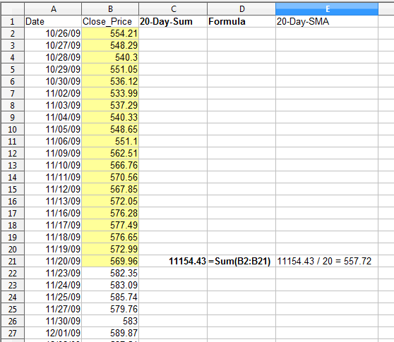
Figure 1 - Base Setup
This shows the base case in which we have to do an initial summation of the close price in the first 20 rows. Remember for this solution, focus on the Sum, not on the average. The 20 day SUM for 11/20/2009 is 11154.43. Now let's move to the next trading day - 11/23/09:
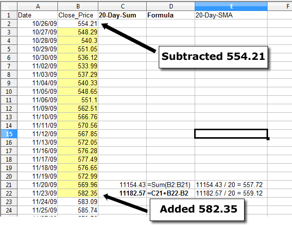
Figure 2 - First Iteration
In order to calculate the Sum this time, we no longer need 20 data points - we only need three: the previous day's sum (C21), the current close price (B22), and the close price from 10/26/2009 (B2). Plugging it into our formula, we get:
Current Sum
= Previous Sum(11154.43) + Current Close Price(582.35) - Close Price from 20 Days Ago (554.21)
= 11182.57
All we have to do is divide this number by 20, and we get our 20 day average for 11/23/09 ($559.12). Let's move it forward once more...
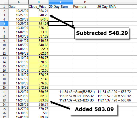
Figure 3 - Second Iteration
At this point you should start to see the "the sliding window" as we iterate through the rows. Feel free to try this iteration with the formula we used before and the data in Figure 3. Hopefully the pattern has now become apparent as we keep iterating through the rows. Taking this into consideration, let's return to the SQL and modify our #mod_goog_data table with one extra field containing the close price from 20 trading days prior:
--drop table #mod_goog_data //drop table if necessary

--Create a CTE worktable t1 to allow us to refer to the n
--field in order to perform a join
with t1 as (select row_number() over (order by quote_date) n
,quote_date
,close_price
from #google_stock)
    select a.n
       ,a.quote_date
       ,a.close_price
       ,CAST(null as decimal(8,2)) [sma]
       --add the close_price from 20 row prior to this one
       ,CAST(b.close_price as decimal(8,2)) [20_day_old_close]
into #mod_goog_data
from t1 a
        left join t1 b
        on a.n - 20 = b.n
With this new #mod_goog_data table, we now have access to 2 of the 3 data points in each row; however we still need data from the previous row. Luckily, we can take the useful information provided by Jeff Moden in his article about Running Totals (make sure you read all the rules before you attempt this) and setup an update statement which would allow us to calculate the the 20 Day SMA in one pass (after we collect the initial 20 day sum):
declare @intervals int, @initial_sum decimal(8,2)
declare @anchor int, @moving_sum decimal(8,2)
set @intervals = 20

 --Retrieve the initial sum value at row 20
 select @initial_sum = sum(close_price)
    from #mod_goog_data
    where n <= @intervals

 update t1
    --case statement to handle @moving_sum variable
    --depending on the value of n
   set @moving_sum = case when n < @intervals then null
     when n = @intervals then @initial_sum
     when n > @intervals then
                        @moving_sum + [close_price] - [20_day_old_close]
     end,
sma = @moving_sum/Cast(@intervals as decimal(8,2)),
@anchor = n    --anchor so that carryover works
from #mod_goog_data t1 with (TABLOCKX)
OPTION (MAXDOP 1)

  select quote_date
   ,close_price
   ,sma from #mod_goog_data
Even though we are executing 3 separate statements for this solution, each only performs 2 logical reads. Furthermore, our main update only requires a single pass to calculate the 20-Day-SMA. I think we can agree that you cannot get much better performance than this. Again make sure you read Jeff's Article before you proceed. If you are uncomfortable using Jeff's running totals solution, I would recommend sticking to the solution in strategy #1. Theoretically Recursive CTE's should work well with this type of problem, but all my testing has provided weaker performance - it takes longer, and does a lot more logical reads than the solution in Strategy #1.
Exponential Moving Averages
Building upon our solution for SMA's, we can actually use the same strategy to calculate EMA's. Exponential averages are slightly different in that it puts more weight on the more recent data, and less on the older data. In calculating the EMA, unlike the SMA (which algorithms relies on the last 20 days), the EMA actually only needs the previous row's EMA, and the current close price. Here is the formula:
EMA = (Close Price * K) + (Previous EMA)*(1 - K)
K = 2/(1 + N)
N = Number of Periods
The EMA is most commonly used to calculate a technical indicator called the Moving Average Converenge / Divergence (MACD). Like the SMA, it is also a trend following indicator and is used to determine the market's momentum (here is more info from Wikipedia about MACD). The formula for the MACD is simply:
MACD = 12 Day EMA - 26 Day EMA
In our example we will calculate both the 12 day and 26 day EMA to provide a practical example. Since calculating the EMA requires the previous day's EMA value, we must setup a base case in order to generate the very first EMA value. This can be done simply by calculating a regular average of all the days prior to our first EMA calculation. If all of this is a lot to grasp, don't worry it is actually quite simple. Again, here is an example with a spreadsheet for the 12 day EMA:
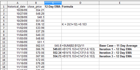
In the 11th data row (D12), the initial average is done by calculating the first 11 close prices, and dividing by 11 (although in the spreadsheet this appears in the12 Day EMA column, in reality we do not want that value to appear to the user, as it is not a true EMA). Once we get to the 12th data row (D13), we see the first iteration of the EMA formula being used (K has been replaced with .153 per the formula in cell D6). From this point on, EMA formula is used until we reach the end of the dataset. A similar method is used to calculate the 26 day EMA; the only difference is that it would start at the 25th data row to find the 25 day average, and that K would be calculated using N = 26.
First let's recreate our #mod_goog_data table to use for calculating the two EMA metrics:
--drop table #mod_goog_data //drop table if necessary

--Setup our Working table for EMA's
select row_number() over (order by quote_date) n
,quote_date
,close_price
,CAST(null as decimal(8,2)) [ema12]
,CAST(null as decimal(8,2)) [ema26]
into #mod_goog_data
from
 #google_stock

 create clustered index ix_n on #mod_goog_data(n)
Again since MACD is a simple subtraction of 12 day EMA minus 26 day EMA, we can calculate the MACD on the fly when we select the values from the table. Now to begin calculating the EMA, we first calculate the initial averages (11 day average and 25 day average). Once we have that, we can do the carryover update just like we did for the SMA (updating 2 fields this time instead of one).
--declare variables needed
declare @ema_1_intervals int, @ema_2_intervals int, @K1 decimal(4,3), @K2 decimal(4,3)
declare @prev_ema_1 decimal(8,2), @prev_ema_2 decimal(8,2), @initial_sma_1 decimal(8,2), @initial_sma_2 decimal(8,2)
declare @anchor int

--Setup the default MACD intervals
set @ema_1_intervals = 12
set @ema_2_intervals = 26
set @K1 = 2/(1 + @ema_1_intervals + .000)
set @K2 = 2/(1 + @ema_2_intervals + .000)

--Capture the averages prior to the start of the EMA interval period
select @initial_sma_1 = avg(case when n < @ema_1_intervals then close_price else null end),
@initial_sma_2  = avg(case when n < @ema_2_intervals then close_price else null end)
from #mod_goog_data
where n < @ema_1_intervals or n < @ema_2_intervals

--Carry over update statement
update t1
set
@prev_ema_1 = case when n < @ema_1_intervals then null
when n = @ema_1_intervals then t1.close_price * @K1 + @initial_sma_1 * (1-@K1)
when n > @ema_1_intervals then t1.close_price * @K1 + @prev_ema_1 * (1-@K1)
end,
@prev_ema_2 = case when n < @ema_2_intervals then null
when n = @ema_2_intervals then t1.close_price * @K2 + @initial_sma_2 * (1-@K2)
when n > @ema_2_intervals then t1.close_price * @K2 + @prev_ema_2 * (1-@K2)
end,
ema12 = @prev_ema_1,
ema26 = @prev_ema_2,
@anchor = n --anchor so that carryover works properly
from #mod_goog_data t1 with (TABLOCKX)
OPTION (MAXDOP 1)

select quote_date, close_price, ema12, ema26, ema12-ema26 macd  from #mod_goog_data
Like with the SMA solution, we have a negligible number of logical reads - a very fast & efficient solution. Of course, anyone who is familiar with the MACD knows it is usually accompanied with a 9-Day EMA of the MACD value in order to measure divergence and pinpoint momentum shifts. Using the tools provided in this article, you'll find it very easy to calculate.
Again if you are uncomfortable using this Running Totals method, unfortunately this time you cannot use a cross join to calculate the EMA. Remember the formula requires the previous day's EMA, so the solution must have a means of carrying over the previous row's values. Unfortunately that leaves either using a Recursive CTE or a Cursor; with those choices, I would probably just revert to calculating the EMA on the client side.


