Introduction

In Part I we learned why Microsoft integrated R and SQL Server. We also learned about the three major R distributions (OSR, MRO and MRS) available today and also their capabilities.

In this part of the series, we will look at some context under which the R distributions could be used selectively by a data scientist to build a predictive model. The discussions will explore and look at the advantages and disadvantages of three major R execution scenarios showcasing the benefits of Microsoft R implementation, especially how ScaleR (ScaleR functions and algorithms) scales R computations out-of-memory.

Context I:

We will look at how the free distributions of R (OSR, MRO) are traditionally used on a local workstation employing standard R implementations. Here the R computations are in-memory, ideal for small data sets. Note that OSR is single threaded. By default MRO is also single threaded but if you install the optional Intel Math Kernel Library (MKL) with MRO the standard R functions are replaced with multithreaded versions.

Context II

We explore how ScaleR could be used to speed up execution on a local work station. Like the first scenario, execution is memory bound, but ScaleR enables multi-threading (currently only up to 2 threads) and it is able to analyze data blocks at a time in parallel. These High Performance Computing (HPC) capabilities helps scale computations without increasing memory. Also, ScaleR could be used to significantly reduce the size of datasets enhancing in-memory computation performance.

Context III

The third context will focus on analyzing SQL Server data remotely. This is a scenario where data in SQL Server running R Services is analyzed in-database on the server. Here, computations are performed at the location of the data. Unlike the memory bound analysis in the previous contexts, computations with MRS and ScaleR in a remote compute context enables full parallel threading & processing. This context could scale to really Big Data computations remotely and distribute them across a cluster of computers (nodes) if available on RDBMs, EDWs, Hadoop and the Cloud.

To follow the examples, I recommend starting with the free Microsoft R Client especially those new to Microsoft R. It gives you Microsoft R Open (MRO) with full support of all base R functions so that you can write R-only solutions, but it also ships with Microsoft R proprietary packages, including the new MicrosoftML package, olapR, mrsdeploy, and the RevoScaleR packages which exposes the ScaleR. You can integrate it with an R IDE of your choice, e.g. Rstudio or R Tools for Visual Studio (RTVS). We will need to run R code in SQL Server, be sure to install R Services as described here.

In the examples I will use the RStudio IDE on my local machine which is running the Microsoft R Client.To test the third scenario, I will connect to a remote SQL Server running R Services. All R and SQL script used for the exercises that follows are in the attached files.

Intro to Data Science Concepts

I titled the series "Advanced Analytics with SQL Server and R…." because with SQL Server and R ( or with only SQL Server today) one could accomplish many Advanced Analytics exercises in Data Science including data preparations, exploratory data analysis, statistical modelling, machine Learning and many more (as outlined on figure1 and figure6 in Part I of the series).

Predictive Analytics

Predictive Analytics is a comprehensive exercise that comprises of many phases. Normally the objective is to be able to predict a response variable using selected predictors as we will see in the example that follows. Predictive modeling problems are mostly defined by their width i.e. the number of potential predictors (columns) and their depth or number of observations or cases (no of rows) in the data set. It is usually the number of potential predictors that gives Data Scientist and analysts the most grief. Depending on the domain or vertical there could be could be thousands of predictors, most of them with weak relationships to the response variable. In the exercises that follow we will be fortunate because we will use about 12 selected predictor out of only a handful. A Predictive Analytics problem for a manufacturer that a team and I worked on had over 1500 predictors. Theerefore the bulk of Predictive modeling process could often involves finding good subsets from numerous predictors.

Note that depending on the business or analytics objectives, a data scientist could be call upon to build various other types of models, a scope too big to discuss here. Predictive Models which are as a result of Predictive Analytics exercises are usually algorithmic models. These models are not used for inferences like other statistical models therefore the way the predictors interact with the response variable is of not much importance. Normally the objective is to find the model that can make the best prediction.

At a high-level, the three major phases in a Predictive Analytics iterative lifecycle are as summarized in the steps in Figure 1 below;

Figure 1: Showing a typical Predictive analytics lifecycle.

The Preparation phase is where the data is first taken in, transformed, cleansed and denormalized. After this stage the data is profiled, explored and visualized. Between 50 to 80 percent of a Data Scientist time could be spent on the data preparation phase.

The Modeling phase is the where the useful subset of predictors and algorithm are selected. Also accomplished alongside in this phase is model testing and validation of data before the model deployed to the operationalization phase.

The Operationalization phase is the phase where the selected model is scored, visualized, measured and then used for predictive analytics.

Note that the process is iterative and continues, especially as more data becomes available.

R and SQL Server Exercise

The previous section tried to put Predictive Analytics endeavors into perspective. In this section we will focus on the Predictive Modeling objectives that we will use to address the three execution contexts outlined under the introduction section above.

The Predictive Analytics Objective

Let's assume we work for a retailer, Adventure Works, who sells bicycles and parts globally on-line and through other channels. They want to grow the business in the US, so they want us to build a model that can predict if a potential on-line customer is likely to buy a bicycle or not. The objective is to use historical data of customers in the US who bought items on-line to build the Predictive Model.

Feature selection

Based on the objectives above, we will assume that the table, dbo.InternetSalesUS (generated from the view in the script attached), represents the subset of customer features that will be useful for making such a prediction. The subset of selected features are: Marital Status, Gender, Yearly Income, Total Number of children, number of children at home, education level, occupation, Home Owner, number of cars owned, commute distance, age and the amount of items bought.

Table 1 below shows a snapshot of the customer features we will use in the modeling process. The binary column, BikeBuyer, represents the response variable; 1 in the column indicates that the customer bought a bike, 0 indicates that the customer did not buy a bike.

Table 1: Showing snap short of the subset of customer features selected to build the predictive model.

Model selection

In a predictive modeling exercise, normally many models are trained using different algorithms and one of the models is selected after some evaluations to determine which of them performs best. Because the main objectives of this article is to showcase the three execution scenarios, the exercises and code that follows will just demonstrate fitting only one algorithm (Logistic Regression) to the training data in all three contexts.

R Code Steps

The terse R code under all code Listings for each execution context will generally consist of four steps as numbered below;

1. Load required packages and define global variables.
2. Connect to SQL Server and query to return the identified subset of customer features.
3. Split the dataset into a training and testing sample sets.
4. Fit a Logistic Regression Model to the training data.

Execution Context I: Traditional R Application

In this section we will demonstrate a scenario where a Data Scientist or an Analyst will to connect to a remote SQL Server Database and extracted data into R on a workstation using either of the free R distribution (OSR and MRO). All R code under this context employs standard R implementations therefore all R computation and are in-memory.

Note that for standard R implementations OSR is single threaded but if you install the optional Intel Math Kernel Library (MKL) with MRO, the standard R implementations are replaced with multithreaded versions and could speed up computations. As shown on Figure 2 below the if you connect to a SQL Server database remotely, the data is brought to the local workstation and all the work is done on the local machine.

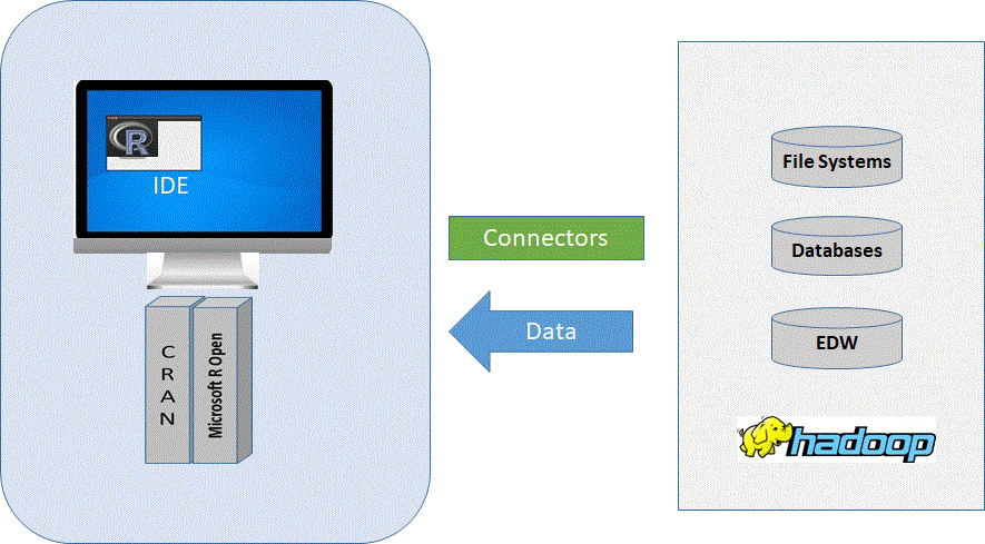
Figure 2: Showing execution context of standard R implementations.

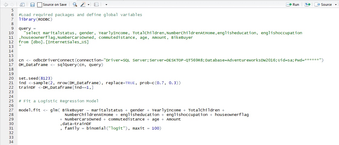
Listing 1 below shows the R code demonstrating the four steps in the predictive modeling process for this scenario.

Listing 1:

R Code explained

The R code for the four step process is shown in Listing 1 is explained below.

• The code initially loads required libraries and functions by calling RRODBC package. A variable with the query string is also defined.
• The odbcDriverConnect function of RODBC package is used to define a connection to a SQL server database and the sqlQuery function of RODBC package is used to send the query and return data into a R dataFrame on local workstation.
• In the following step the returned dataset in the Dataframe is splt (70:30 %) into a training and testing sample.
• Finally, a logistic regression model is fitted to the training data using the glm() algorithm and the training Dataframe.

Advantages

Under this context, standard R implementation enables very fast computations especially where smaller data sets fits in-memory. The Data scientist working on a local workstation also have a lot of control over the environment and the flexibility to apply a lot community R functionality.

Disadvantages

On the other hand the context limits large data computation where data does not fit in-memory. Extraction of data into R locally across networks leads to wasteful data movement and also poses security vulnerability. Operationalization of predictive models under this context may require a lot more work without and also lacks commercial supports as offered by Microsoft R.

Context II: Using ScaleR to enable Parallelization Locally

In this section will demonstrate a scenario where a data scientist will to connect to a SQL Server Database and extracted data into R on a workstation running the R Client (which enables ScaleR on MRO). Even though computations are in-memory like the first scenario, ScaleR enables this execution context to scale to larger datasets because it is able to analyzes data blocks at a time in parallel. ScaleR is also used here to first compress the data significantly which help speed up computations in-memory.

As shown in Figure 3 below and like the first scenario, the data is brought to the local workstation and all the work is done on the local machine.

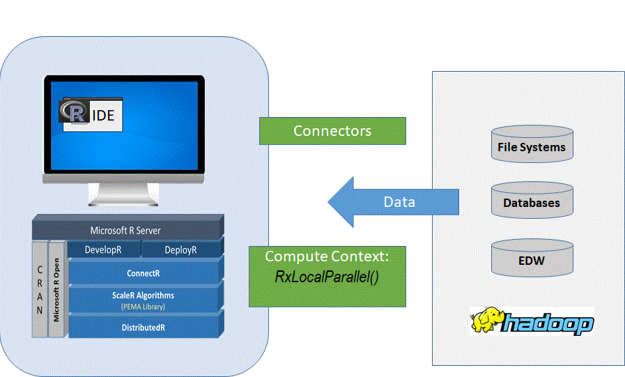
Figure 3: Showing execution context where ScaleR functions and algorithms can be used to speedup R computation in a local context.

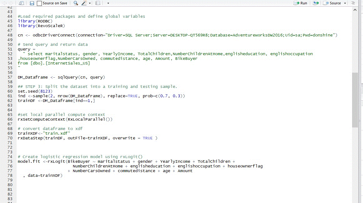
Listing 2 below shows the R code demonstrating the four steps in the predictive modeling process for this scenario.

Listing 2:

R Code Explained

The R code for the four step process under this scenario is shown in Listing 2 is explained below.

• The code initially load required libraries and functions by calling RRODBC package. A variable with the query string is also defined.
• The odbcDriverConnect function of RODBC package is used to define a connection to a SQL server database and the sqlQuery function of RODBC package is used to send the query and return data into a R dataFrame on local workstation.
• In the following steps the returned dataset in the dataframe is splt (70:30%) into a training and testing sample. Note that the Dataframe of the training set is further converted to an XDF output file format using a ScaleR function, rxDataStep. Microsoft R function that enables parallelization are prefix with rx. To use these functions, first, the context of execution is defined with the function rxSetComputeContext. The rxLocalParrallel function signals that all ScaleR parallelization functions should be executed in a local context.
• Finally, a logistic regression model is fitted to the training data using the ScaleR algorithm rxlogit and the training XDF file.

Advantages

Unlike the first scenario, this execution context scales to larger datasets because ScaleR enables HPC capabilities that analyzes data blocks at a time and in tparallel. secondly, the rxDataStep functions used reduces the size of datasets by converting it to XDF output file format which are 5 times smaller than say csv files enhancing in-memory computation performance. ScaleR uses c++ to build algorithms/compiled execution as opposed to interpreter which are often slow than the compiled languages because of a number of reasons.

Disadvantages

Like context I, extraction of data into R locally across networks leads to wasteful data movement and also poses security threat. The CPU centric HPC performance capabilities enabled by ScaleR in this context is still dependent on local memory and a single disks and therefore does not scale to really Big Data analysis.

Context III: Remote Execution with ScaleR.

In this section we will demonstrate a scenario where a data scientist will to connect to a SQL Server running R Services remotely. Unlike the previous two scenarios remote execution using MRS and ScaleR enables R to automatically computate data blocks at a time in parallel on available cores and also able to automatically distribute computations across multiple computers (nodes) in clusters where available.

As shown of Figure 4 below and unlike the previous two scenario, the data stays on the remote server and the work is done on the server.

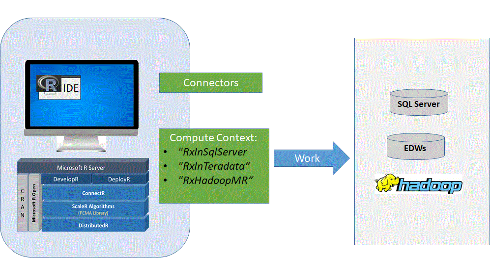
Figure 4: Showing execution context using ScaleR functions for full parallelization and distributed workloads.

Listing 3 below shows the R code demonstrating the four steps in the predictive modeling process for this scenario.

Listing 3:

R Code Explained

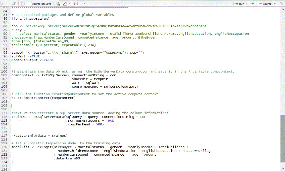
The R code for the four step process under this scenario is shown in Listing 3 is explained below.

• The code initially loads required libraries and functions by calling RevoScaleR package. Besides the query and connection strings, a few other variables used to create the compute context are also defined;

sqlShareDir is the temp directory path the Set Compute Context will use to serialize R objects back and forth between your workstation.

sqlWait stores logical parameter value. If TRUE, the job will be blocking and will not return until it has completed or has failed. If FALSE, the job will be non-blocking and return immediately, allowing you to continue running other R code. The object

sqlConsoleOutput stores the value that causes the standard output of the R process started by SQL Server to be printed to the user console or not.

The next lines instantiate the data object, using the RxSqlServerData constructor and save it in the R variable compcontext. We then call the function rxSetComputeContext to set the active compute context. Next, we can create a SQL Server Data Source, using the query for the training dataset we defined.

Note that the Data Source is just a reference to the result dataset from the SQL query. The data is not actually pulled into the local environment. Because we set compute context to the SQL Server computer, the data stays on the server and we have only a pointer to it in the R code.

Unlike the previous scenarios where we split the dataset into Training and Test set with R, here we split the data on SQL server using the T-SQL tablesample function as shown in the query variable.

Finally, a logistic regression model is fitted to the training data using the ScaleR algorithm rxlogit and the training Data Source.

Advantages

Unlike the local execution contexts in the first two scenarios, remote execution enabled by MRS and ScaleR perform computations where the data is situated. This eliminates wasteful data movement across networks and also limits security concerns. This context provides even faster computations facilitating speedy real-time scoring and able to scale to big data. This is made possible because the core ScaleR under this execution context has the ability to automatically compute data blocks at a time in parallel on available cores and also able to automatically distribute computations across multiple computers (nodes) in clustered environments where available. The R Server also enables the instant deployment and easy consumption of R analytics with enterprise-grade security and commercial support.

Disadvantages

Under this context R does not have control on the remote execution Grids; RDBMs, EDWs, Hadoop and Cloud.

Write Once-Deploy Anywhere

In Microsoft R architecture Write Once-Deploy Anywhere (WODA) concept rely on the fact that, with MRS, models you build can be deploy on-premises, in the cloud or even to Linux and Hadoop systems as shown in Figure 5 below.

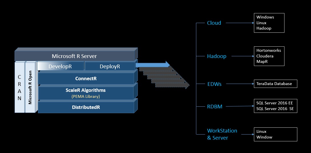
Figure 5: Showing the various R deployment environments enabled by MRS.

Notice that in all three execution scenarios the actual code base does not change that much, such that, with slight modifications, the code you develop on the desktop can be deployed in many environments.

Conclusion

Standard R implementation is capable of fast computations ideal for small data sets that fit in-memory. On the other hand Microsoft R implementation comes with HPC functions and algorithms that automatically compute lots of small chunks of data at a time in parallel on available cores helping to scale computations linearly. Backed by MRS, these Parallel External Memory Algorithm’s (PEMA’s) further enables High Performance Analysis (HPA) capabilities that help scale computations to really big data by using more computers (nodes). HPA capabilities increase scale and speed by turning to I/O bounding when data cannot fit into memory. The process takes advantage of memory caching on the nodes and focuses on feeding data to the cores—on multiple disk I/Os in addition to the in-built efficient threading and data management in RAM.

We learned that Microsoft R's ScaleR implementation consist of such functions and algorithms written to automatically compute in parallel on available cores . As we demonstrated in context II, ScaleR have limiting capabilities and thus it is not able to Scale to really Big Data computations in some local context. On the other hand when you employ the MRS, ScaleR ( which is built on DistributedR) enables remote computations that permits full parallelization and is also able to automatically distribute computations across multiple computers (nodes) on a cluster or in the cloud, addressing the limiting speed and capacity issues with Big data analysis.

Note that for Big Data analysis there are a lot of other things you might want to consider besides what we discussed here, but you may want to consider Microsoft R implementation over Standard R implementation based on some of the benefits we've highlighted above.

Next

In Part III, the next and final part of the series, we will do sample walk through on how to do Advanced Analytics (Predictive Modeling) with R, entirely in SQL Server using TSQL; which is probably the biggest essence of the SQL Server and R integration.We will see how SQL Server support entire in-database advance analytics Lifecycle by building & deploying and operationalizing a predictive Model.