In this Level, we will continue the introduction to the general MDX member functions I began in Level 5: Members, and an Introduction to the MDX Members Functions. In particular, we’ll continue our focus on the “family” basic member functions, this time taking up the Ancestor() and .FirstChild functions. We’ll discuss the syntax underlying each, together with the information it returns. We’ll then get some hands-on exposure to each function, creating queries that put it to work and then analyzing the data set that the queries return, to confirm our understanding of the use and operation of the respective function.

Let’s take a look at each of these “family” functions individually, beginning with the Ancestor() function.

The Ancestor() Function

As we’ll soon see, the Ancestor() function retrieves the member, at the specified level, or at the specified distance, that is the ancestor (the parent, parent of parent, or higher) of the source member under consideration. Like the .Parent and .Children functions, it travels within a “vertical” scope, moving up between hierarchical levels from the member to which it is applied.

Differences exist between the functions, as we would expect. A mechanical difference lies within the simple fact that the Ancestor() function is applied differently than the .Parent and .Children functions, in that it is not “appended” to the source member. The source member is placed within the parentheses to the right of the word “Ancestor,” as shown in the following:

Ancestor(member, level)

or

Ancestor(member, distance)

Another difference is that the Ancestor() function can contain the aforementioned level, or distance, component (represented by the second argument within the parentheses of the first and second options shown above, respectively).

An illustration of the Ancestor() function (using a level target) follows:

SELECT
{[Measures].[Internet Sales Amount],
[Measures].[Internet Order Quantity]} ON COLUMNS,
{(ANCESTOR(
[Date].[Calendar].[Month].[March 2007],
[Date].[Calendar].[Calendar Quarter]))} ON ROWS
FROM
[Adventure Works]

The result dataset returned when executing the above would appear as depicted here.

Illustration 1: Example Result Dataset from Using the Ancestor() Function

(In the illustration above, a target level that equaled the level of the member within the function would have returned the member itself.)

If a distance target is specified, the distance component is represented by a number. The number represents “number of hierarchical steps above the source member.” The member itself is returned if the number is zero, reasonably enough.

Let’s reinforce our understanding of how the function operates by using it in a couple of queries. We will, as usual, work with the MDX Query Editor in SSMS. If you are not sure how to set up SSMS in Analysis Services to access the Adventure Works DW 2008R2 database, then click here for guidance.

We will use the second of the syntax structures (Ancestor(member, distance) in our first example.

Let’s assume that we have been given a business requirement by a hypothetical client: We have been asked by our analyst colleague in the Sales and Marketing department of the Adventure Works organization to provide both the total Internet Sales Amount and Internet Order Quantity for the ancestor member one level above the source member that we used in the Syntax illustration above. (We’ll handle measure specification via the slicer enacted by the WHERE clause). We are asked to provide the information in a two-dimensional grid, with the measures in the column axis and the specified month of interest (the Ancestor of March 14 2008), in the row axis.

Type (or copy and paste) the following query into a blank Query pane:

-- SMDX007-001: Using ANCESTOR() Function in Row Specification,
-- “Distance” target
SELECT
{[Measures].[Internet Sales Amount],
[Measures].[Internet Order Quantity]} ON AXIS(0),
{(ANCESTOR(
[Date].[Calendar].[Date].[March 14, 2008],1))}
ON AXIS(1)
FROM
[Adventure Works]

Here, we’re specifying two measures, Internet Sales Amount and Internet Order Quantity in our columns, and don’t require the slicer specification (WHERE). We are also using the Ancestor() function with the distance target of Month in the Calendar hierarchy of the Date dimension. Because we specify the Date level, with March 14, 2008 as the source member, we would expect to see the month of March (for calendar year 2008) in the result dataset. We will not be disappointed in our expectations.

The query appears within the Query pane.

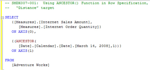
Illustration 2: Initial Query, using Ancestor(), in the Query Pane

Click the Execute (!) button in the toolbar.

The Results pane is populated with the dataset.

Illustration 3: The Initial Query Results in the Results Pane

The results dataset displays the totals at the level of the month of March, 2008, the ancestor (with a “distance” of one (1) “generation”) of the date March 14, 2008 at the hierarchical level of Month of the Date dimension.

Save the query by selecting File Save MDXQuery1.mdx As …, naming the file SMDX007-001.mdx, and placing it in a meaningful location.

Now let’s illustrate the operation of the Ancestor() function once again, with another example, this time using the level target variation of the function. Let’s say the next client request surrounds the ancestor of a Postal Code, residing at the State-Province level of the Customer dimension (Customer Geography hierarchy).

Select File New from the top menu.

Select Query with Current Connection from the cascading menu that appears next.

Type (or copy and paste) the following query into the Query pane:

-- SMDX007-002: Using ANCESTOR() Function in Row Specification,
-- “Level” Target
SELECT
{[Measures].[Internet Sales Amount],
[Measures].[Internet Order Quantity]} ON AXIS(0),
{(ANCESTOR(
[Customer].[Customer Geography].[Postal Code].[30253],
[Customer].[Customer Geography].[State-Province]))} ON AXIS(1)
FROM
[Adventure Works]

Here, as in the previous example, we’re specifying two measures, Internet Sales Amount and Internet Order Quantity, in our columns, and don’t, once again, require the slicer specification (WHERE). We are also using the Ancestor() function with the level target of State-Province in the Customer Geography hierarchy of the Customer dimension. Because we specify the Postal Code level, with 30253 as the source member, we would expect to see the U.S. state of Georgia in the result dataset. Again, our expectations will prove to be correct.

The query appears within the Query pane.

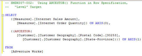
Illustration 4: Second Query, using Ancestor(), in the Query Pane

Click the Execute (!) button in the toolbar, once again.

The Results pane is populated.

Illustration 5: The Query Results, via Ancestor() – “Distance” Mode

The results dataset displays the totals for Georgia, the ancestor of Postal Code 30253 at the level of State-Province in the Customer Geography level of the Customer dimension.

Save the query by selecting File Save MDXQuery2.mdx As …, and naming the file SMDX007-002.mdx.

Now that we’ve seen how to use the Ancestors() function, let’s move to another “family” member function, .FirstChild.

The .FirstChild Function

The .FirstChild function returns the first child of a specified member. Let’s move directly to an illustration to gain an understanding of just what we mean by a “first child.” I have chosen the Date dimension within the Adventure Works sample cube, for this illustration, because we all understand the Calendar hierarchy (which will make a grasp of the core concepts less subject to being fettered by a need to study a hierarchical structure within the sample database). The example to which I refer appears below.

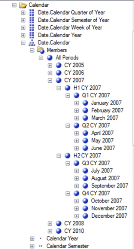
Illustration 6: Date.Calendar Hierarchy, Showing CY 2007, Expanded to Month Level

Syntactically, the .FirstChild function is appended to the right of the member, as shown in the following:

<member>.FirstChild

A simple example of the .FirstChild function in action follows:

SELECT
{[Date].[Calendar].[Calendar Year].[CY 2007].FIRSTCHILD}
ON COLUMNS
FROM
[Adventure Works]
WHERE
([Measures].[Internet Sales Amount])

The result dataset returned would appear as shown:

Illustration 7: Example Results Dataset from Using the .FirstChild Function

A look at the Date hierarchy for the source member (CY 2007) within the .FirstChild function above will make the illustration more meaningful. In Illustration 10 below, we see that H1 CY 2007 is a member of the Semesters / Half-Year sublevel of the Calendar Year level, within the Date.Calendar dimension hierarchy. The order of the members within the database determines the status of H1 CY 2007 as “first:” H1 CY 2007 is the child of the CY level 2007, and as it is “first in line,” it is returned via the .FirstChild function.

Here’s a graphic presentation:

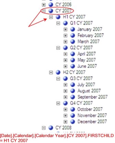
Illustration 8: [Date].[Calendar].[Calendar Year].[CY 2007].FIRSTCHILD is H1 CY 2007

In the simple example above, we can easily see that the parent member is CY 2007.

We touched upon the WHERE clause in Level 6: Member “Family” Functions: .Parent and .Children, in a discussion of the .Parent function. As we discussed at that point, the WHERE clause is optional; it specifies the Slicer Dimension, and limits the data returned to specific dimension(s) or member(s). The WHERE clause in our illustration above restricts the data extracted for the axis dimensions to a specific member of the Measures dimension, Internet Sales Amount.

Let’s solidify our understanding of how the .FirstChild function operates by working within another simple illustration, and extending that illustration to other basic examples that actually add the .FirstChild function to a given member. Let’s assume that our client colleague has returned with another request: he’d like to see the total Internet Sales Amount for each of the Product Categories for the first Semester of Calendar Year 2008. He explains that the ultimate objective will be to parameterize the Year, and to select the first semester based upon the year selected.

We recognize this this business requirement as an opportunity to demonstrate the use of the .FirstChild function (because the first semester of any given Calendar Year in the Adventure Works cube structure is the “first child” of the Year level of the Date dimension – Calendar hierarchy) to the client organization, and proceed to do so in the following steps.

Select File New from the top menu.

Select Query with Current Connection from the cascading menu that appears next, once again.

Type (or copy and paste) the following query into the Query pane:

-- SMDX007-003: Basic Use of .FIRSTCHILD
SELECT
{[Date].[Calendar].[Calendar Year].[CY 2008].FIRSTCHILD}
ON AXIS(0),
{[Product].[Category].MEMBERS} ON AXIS(1)
FROM
[Adventure Works]
WHERE
([Measures].[Internet Sales Amount])

he query appears in the Query pane, once again.

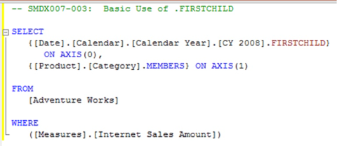
Illustration 9: The Query in the Query Pane

Click the Execute (!) button in the toolbar, as before.

The results appear in the Query pane, as soon as Analysis Services fills the cells that it determines to be specified by the query.

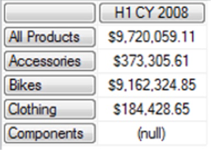
Illustration 10: Results of the Query Using .FirstChild()

The query delivers the results that were requested by the information consumer.

Save the query by selecting File Save MDXQuery3.mdx As …, and naming the file SMDX007-003.mdx.

Let’s examine a graphical illustration of the operation we have just witnessed, via the results returned by our query, of the .FirstChild function. A quick look at the hierarchy illustrates the relationships between the members and levels under consideration that we saw earlier:

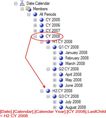
Illustration 11: The Hierarchy under Consideration

As our straightforward example makes obvious, the “first child” of level member [Date].[Calendar].[Calendar Year].[CY 2008] is H1 CY 2008. (As to the use of the .Members function, recall from Level 5: Members, and an Introduction to the MDX Members Functions that the .Members operator gives us the members of the dimension / dimension hierarchy.)

Let’s try another query using .FirstChild. This time, we’ll write a basic query to return total Internet Sales Amount by Product Category, once again, but by quarter, in this exercise, instead of semester (that is, each of the quarter children of semester member H1 CY 2008). Recall our discussion surrounding the .Children function in Level 6: Member “Family” Functions: .Parent and .Children.

From the use of .Children we will enumerate the quarters contained within semester H1 CY 2007, which we saw earlier was the first child of member CY 2008 of the Date dimension, Calendar hierarchy. Our objective will be to create a column for each quarter in semester H1 CY 2008 and a row for each Product Category.

Select File New from the top menu, as we did earlier.

Select Query with Current Connection from the cascading menu that appears next, once again.

Type (or copy and paste) the following query into the Query pane:

-- SMDX007-004: .FIRSTCHILD with .CHILDREN to Descend Another "Generation"
SELECT
{[Date].[Calendar].[Calendar Year].[CY 2007].FIRSTCHILD.CHILDREN} ON AXIS(0),
{[Product].[Category].MEMBERS} ON AXIS(1)
FROM
[Adventure Works]
WHERE
([Measures].[Internet Sales Amount])

The query appears in the Query pane, once again.

Illustration 12: The Query with .FirstChild and .Children Combination

Click the Execute (!) button in the toolbar atop the Management Studio, once again.

The retrieved data appears in the Results pane.

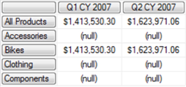
Illustration 13: The Query Results Dataset, via the .FirstChild and .Children Combination

The query delivers the totals for the enumerated members (including, of course, the “All” member) of the Product Category level of the Product dimension, for each of the two children (that is, Q1 CY 2007 and Q2 CY 2007) of the first child (H1 CY 2007) of the 2007 member of the year level of the Date dimension.

We see that we have obtained a summary for each of the Product Category members’ Internet Sales Amount, for each of the two quarters of the first semester of CY 2007, because we affixed the .FirstChild function to the CY 2007 year level of the Date.Calendar dimension hierarchy, and then appended the .Children function to the .FirstChild function. As we determined to have been the case in our exposure of the .Parent function in Level 6: Member “Family” Functions: .Parent and .Children, as well as elsewhere, we will find the .FirstChild and other “family” functions even more powerful in later levels of our series, where we employ relative members, such as .CurrentMember. As we’ll discover, the placement of the calculation within which the respective family function is housed will determine its context.

Save the query by selecting File Save MDXQuery4.mdx As …, naming the file SMDX007-004.mdx, and placing it, once again, in a convenient location.

Save the query by selecting File Save MDXQuery6.mdx As …, naming the file SMDX007-006.mdx.

We will continue our examination of the “family” member functions in the next Level of Stairway to MDX.

Summary …

In this Level, we continued the introduction to the general MDX member functions begun in Level 5: Members, and an Introduction to the MDX Members Functions, and continued in Level 6: Member “Family” Functions: .Parent and .Children. In this Level, we continued our focus on the “family” basic member functions, exploring the Ancestor() and .FirstChild functions, discussing for each the syntax within which it is employed, as well as the information it returns and other details. We gained the know-how needed to take advantage of these useful functions through the typical Stairway practice exercises, whereby we constructed queries that used each function, and then examined together the results datasets those queries delivered.