The next version of SQL Server (v11.0), which at the time of the writing of this article is code-named “Denali”, was recently released as beta #3 (otherwise known as Community Technology Preview 3 (CTP3)). As you might expect from a new version of SQL Server, there are several new and enhanced features being added. This article is about the enhancements to the OVER clause and the different functions that can utilize it. (Because this version of SQL Server is a beta product at this point, the information in this article may change when this version is released to RTM. Since the changes described adhere to the ANSI specification, I don’t expect any changes.)
What the OVER Clause is
In relational database systems, the sets of data are by nature unordered. Unless ORDER BY is specified on a query, order of data returned in a query is not guaranteed. The OVER Clause allows you to assign a numerical order to a number of functions within your unordered set. The functionality is further extended to support partitions (groupings) of data, in a specified order, and for a specified range of rows within the partition.
In prior versions of SQL Server (2005, 2008 and 2008R2), the OVER Clause is a partial implementation of the ANSI: SQL 2003 standard. For the Ranking functions (ROW_NUMBER, RANK, DENSE_RANK and NTILE), the PARTITION BY and ORDER BY clauses of the OVER clause are supported. For the Aggregate functions (AVG, CHECKSUM_AGG, COUNT, COUNT_BIG, MAX, MIN, STDEV, STDEVP, SUM, VAR and VARP), just the PARTITION BY clause is supported. The OVER clause does not support the ROWS|RANGE clause to define the rows to include in the window – the entire partition is used.
If you don’t understand how the OVER clause works in the prior versions of SQL Server with the PARTITION BY and ORDER BY clauses, please take a moment to read my article “SQL Server Ranking Functions” where they are explained along with examples of each of these clauses and how they work together. The rest of this article assumes that you have this basic understanding.
How the OVER Clause has changed in “Denali”
To start off with, the syntax is simply:
OVER (
       [ <PARTITION BY clause> ]
       [ <ORDER BY clause> ]
       [ <ROW or RANGE clause> ]
      )
The first change to note is that the PARTITION BY and ORDER BY clauses apply not only to the Ranking functions, but also to the Aggregate functions, the new Analytic functions, and the new NEXT VALUE FOR function (used to generate a sequence).
The second change to note is a new clause – the “ROW or RANGE” clause. It is used to specify which of the rows within the partition are to be used in evaluating the function that is being used with the OVER clause. In BOL, this is further broken down into specifics that make this clause look pretty complicated. Actually, it is relatively simple. You start off by specifying whether the OVER Clause is to use ROWS (for a physical association to the current row), or RANGE (for a logical association to the current row based on the value of the column(s) in the ORDER BY clause). This is followed by specifying the starting point and optionally the ending point of the window to be used with the function. If you use the optional ending point, you will use the “BETWEEN <starting point> AND <ending point>” syntax. If you don’t use the optional ending point, then you will use the “<starting point>” syntax and the ending point will default to “CURRENT ROW”. Each of these methods will be shown in the following examples.
The starting and ending points are specified in one of three ways: UNBOUNDED with either PRECEDING or FOLLOWING, <unsigned value specification> with either PRECEDING or FOLLOWING, or CURRENT ROW.
UNBOUNDED specifies that the window either starts at the first row of the partition (if using PRECEDING), or ends at the last row of the partition (if using FOLLOWING). A different way to think of this is that UNBOUNDED specifies to use all of the rows (or range of values) PRECEDING the current row, or all of the rows (or range of values) FOLLOWING the current row.
CURRENT ROW specifies that the window starts or ends at the current row (with ROWS) or at the current value (with RANGE). It can be used as both the starting and ending point.
<unsigned value specification> indicates the number of rows to precede (PRECEDING) or follow (FOLLOWING) the current row. You are not allowed to use this option with RANGE. If you use <unsigned value specification> FOLLOWING as the starting point, the ending point must also use <unsigned value specification> FOLLOWING. For example, if you were to use ROWS 2 PRECEDING, then for each row the window function is applied to, only the current row and the two rows prior to it are considered for the function.
A few things to remember:
- If ORDER BY is not specified, then the entire partition is used for a window frame.
- If ORDER BY is specified, but ROWS|RANGE is not, then the window frame defaults to RANGE BETWEEN UNBOUNDED PRECEDING AND CURRENT ROW.
- The ORDER BY clause must be specified in order to use the ROWS|RANGE clause.
- Not all functions support the ORDER BY / ROWS|RANGE clauses.
Putting this to some use.
“Wayne, this is all pretty nice. But how do I use it? What use is this to me?” Well, I’m glad you asked.
For the next three samples, I’m going to use the following sample data. This code builds a transaction table of Accounts, Transaction Dates, and Transaction Amounts.
DECLARE @SampleData TABLE (
  AccountId INTEGER,
  TranDate  DATETIME,
  TranAmt   NUMERIC(8,2));

INSERT INTO @SampleData
            (AccountId, TranDate, TranAmt)
     VALUES (1, '20110101', 500),
            (1, '20110115', 50),
            (1, '20110122', 250),
            (1, '20110124', 75),
            (1, '20110126', 125),
            (1, '20110128', 175),
            (2, '20110101', 500),
            (2, '20110115', 50),
            (2, '20110122', 25),
            (2, '20110123', 125),
            (2, '20110126', 200),
            (2, '20110129', 250),
            (3, '20110101', 500),
            (3, '20110115', 50 ),
            (3, '20110122', 5000),
            (3, '20110125', 550),
            (3, '20110127', 95 ),
            (3, '20110130', 2500);
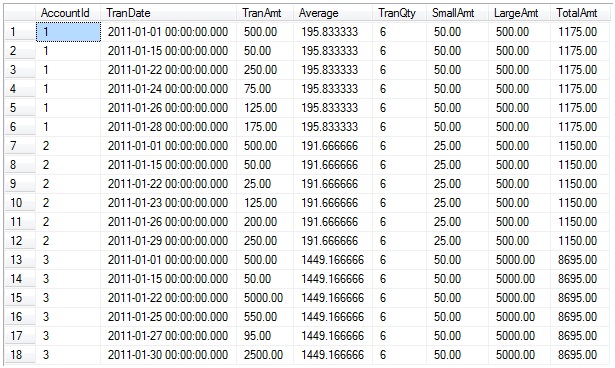
Let’s take a brief detour and look at what the previous versions of SQL could handle. If we consider just the rows for AccountId 1, we see that there are 6 rows. When we partition by AccountId, these 6 rows are the “window” for AccountId 1. The total of the TranAmt for these 6 rows is 1175, the smallest value is 50, the largest value is 500, and the average is 195.83. When we utilize the OVER clause with the AVG, COUNT, MIN, MAX and SUM functions, and if we specify to PARTITION BY AccountId, then we are specifying that for each AccountId we will be perform that functions’ aggregation for the window (for the rows for that AccountId). This aggregation is then repeated for each AccountId. In essence, a series of aggregations are being performed, once for each partition (AccountId).
The pre-“Denali” code for these aggregations utilizing the PARTITION BY clause is:
SELECT AccountId ,
       TranDate ,
       TranAmt,
       -- average of all transactions
       Average  = AVG(TranAmt) OVER (PARTITION BY AccountId),
       -- total # of transactions
       TranQty  = COUNT(*)     OVER (PARTITION BY AccountId),
       -- smallest of the transactions
       SmallAmt = MIN(TranAmt) OVER (PARTITION BY AccountId),
       -- largest of the transactions
       LargeAmt = MAX(TranAmt) OVER (PARTITION BY AccountId),
       -- total of all transactions
       TotalAmt = SUM(TranAmt) OVER (PARTITION BY AccountId
  FROM @SampleData
 ORDER BY AccountId, TranDate;
This “Total Aggregation” query returns the following result set:

As you can see, the aggregations are at the entire partition level – for each partition (AccountId), the aggregations are calculated for each of the rows in that partition, and all of the rows in that partition all have the same values for the aggregation.
Switching back to what “Denali” allows, let’s change this query to use “Running Aggregates” – as we progress to each row, the aggregate function is applied to all of the rows that have been encountered by the partition thus far. We change those aggregations to be “Running Aggregations” by utilizing the ORDER BY clause in the OVER clause. Let’s use the following code:
SELECT AccountId ,
       TranDate ,
       TranAmt,
       -- running average of all transactions
       RunAvg      = AVG(TranAmt) OVER (PARTITION BY AccountId
                                            ORDER BY TranDate),
       -- running total # of transactions
       RunTranQty  = COUNT(*)     OVER (PARTITION BY AccountId
                                            ORDER BY TranDate),
       -- smallest of the transactions so far
       RunSmallAmt = MIN(TranAmt) OVER (PARTITION BY AccountId
                                            ORDER BY TranDate),
       -- largest of the transactions so far
       RunLargeAmt = MAX(TranAmt) OVER (PARTITION BY AccountId
                                            ORDER BY TranDate),
       -- running total of all transactions
       RunTotalAmt = SUM(TranAmt) OVER (PARTITION BY AccountId
                                            ORDER BY TranDate)
  FROM @SampleData
 ORDER BY AccountId, TranDate;
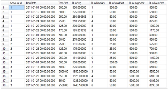
(Remember that when omitting the ROWS|RANGE clause (when you have the ORDER BY clause specified) that the default RANGE for this new functionality is RANGE BETWEEN UNBOUNDED PRECEDING AND CURRENT ROW.) This “Running Aggregation” code produces this result set:

Okay, this shows pretty well how “Running Aggregations” work – each of the aggregate functions is applied to only the rows that have been encountered so far by the ORDER BY clause, and are reset by changes to values in the PARTITION BY clause. Specifically, for the first row the running total is its TranAmt (500), and the running smallest amount is 500. When we go to the second row, the running total adds the current TranAmt (50) for a total of 550, and the smallest TranAmt for this partition is now 50. For the third row, the TranAmt (250) is again added to the running total for a total of 800, and 50 is still the smallest TranAmt. When we move to rows 7 or 13, which are the start of a new partition, everything restarts.
To duplicate the original functionality of the pre-“Denali” aggregations, we could have used RANGE BETWEEN UNBOUNDED PRECEDING AND UNBOUNDED FOLLOWING – or simply just omit the ORDER BY and ROWS|RANGE clauses as I did in the previous example.
Now, let’s dive into the next use: “Sliding Aggregations”. Let’s say that the new requirement is that each of these aggregations is to be calculated on the current row, and for just the two rows preceding it. This requires changing the OVER clause to include the ROWS clause:
SELECT AccountId ,
       TranDate ,
       TranAmt,
       -- average of the current and previous 2 transactions
       SlideAvg      = AVG(TranAmt) OVER (PARTITION BY AccountId
                                              ORDER BY TranDate
                                               ROWS BETWEEN 2 PRECEDING AND CURRENT ROW),
       -- total # of the current and previous 2 transactions
       SlideTranQty  = COUNT(*)     OVER (PARTITION BY AccountId
                                              ORDER BY TranDate
                                               ROWS BETWEEN 2 PRECEDING AND CURRENT ROW),
       -- smallest of the current and previous 2 transactions
       SlideSmallAmt = MIN(TranAmt) OVER (PARTITION BY AccountId
                                              ORDER BY TranDate
                                               ROWS BETWEEN 2 PRECEDING AND CURRENT ROW),
       -- largest of the current and previous 2 transactions
       SlideLargeAmt = MAX(TranAmt) OVER (PARTITION BY AccountId
                                              ORDER BY TranDate
                                               ROWS BETWEEN 2 PRECEDING AND CURRENT ROW),
       -- total of the current and previous 2 transactions
       SlideTotalAmt = SUM(TranAmt) OVER (PARTITION BY AccountId
                                              ORDER BY TranDate
                                               ROWS BETWEEN 2 PRECEDING AND CURRENT ROW)
  FROM @SampleData
 ORDER BY AccountId, TranDate;
(Note that each of these “ROWS BETWEEN 2 PRECEDING AND CURRENT ROW” clauses could have been written as “ROWS 2 PRECEDING”, since CURRENT_ROW is the default ending point if not specified.)
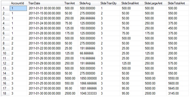
This “Sliding Aggregation” code produces this result set:

As you can see, the values for the aggregate functions change based upon the two rows that are preceding the current row.
Now let’s take a look at the difference between utilizing the ROWS and RANGE clauses. As described above, ROWS is a physical association between rows – Row #1, #2, #3, etc. For RANGE, this is a logical association based on the value of the column(s) in the ORDER BY clause, and all rows with the same value are handled together. For this example, let’s use a simple salary table:
DECLARE @Test TABLE (
    RowID INT IDENTITY,
    FName varchar(20),
    Salary smallint);

INSERT INTO @Test (FName, Salary)
VALUES ('George',       800),
       ('Sam',          950),
       ('Diane',       1100),
       ('Nicholas',    1250),
       ('Samuel',      1250),
       ('Patricia',    1300),
       ('Brian',       1500),
       ('Thomas',      1600),
       ('Fran',        2450),
       ('Debbie',      2850),
       ('Mark',        2975),
       ('James',       3000),
       ('Cynthia',     3000),
       ('Christopher', 5000);
For this example, we will use the SUM function on the Salary column, and we will use the OVER clause with the ORDER BY and both the ROWS and RANGE clauses.
SELECT RowID,
       FName,
       Salary,
       SumByRows  = SUM(Salary) OVER (ORDER BY Salary
                                       ROWS UNBOUNDED PRECEDING),
       SumByRange = SUM(Salary) OVER (ORDER BY Salary
                                      RANGE UNBOUNDED PRECEDING)
  FROM @Test;
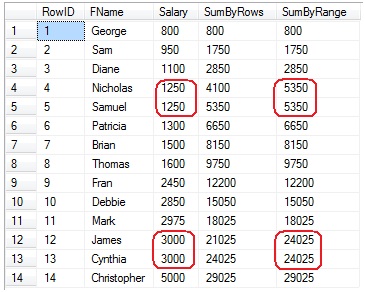
(In this example, since only the starting point is specified, the ending point defaults to the current row.) The result set for this query is:

The SumByRows column produces a running total over the Salary column, in order of the Salary, with the running total being the previous row’s accumulated total plus the current row’s Salary – just like in the “Running Aggregation” example above.
The SumByRange column produces the running totals over all of the rows for each value in the Salary column, with the total for each row being the accumulated total for the previous value of the Salary column, plus the total of all rows that have the same value as the current row. Note rows 4-5 – in the SumByRows columns, row 3’s running total (2850) is added to the row 4’s salary (1250) for a total of 4100, and then for row 5 its salary (1250) is added to 4100 for a total of 5350. In the SumByRange column, the sum of the salary column for all rows with the same salary as in row 4 is added to row 3’s running total, so 2850 + (1250 * 2) = 5350. It is not computed for each row – it is computed for each range of values. The same thing happens for rows 12-13. (Notice that the last of these rows in the SumByRows column is what the SumByRange column has for each of the rows.)
New “Denali” Functions that utilize the OVER clause
In addition to these enhancements to the OVER clause, “Denali” also introduces 9 new functions. Eight of these are Analytic functions, and the ninth is used for sequence number generation. The Analytic functions require the use of the OVER clause, while for the NEXT VALUE FOR function using the OVER clause is optional. Please see the Analytic Functions or NEXT VALUE FOR BOL references for the syntax and usage of these functions.
Thanks for taking the time to read this. I hope that this article makes you yearn for the RTM release of “Denali”!
References
OVER Clause (SQL 2008 R2 BOL) | http://msdn.microsoft.com/en-us/library/ms189461%28v=SQL.105%29.aspx |
OVER Clause (SQL Server “Denali” BOL) | http://msdn.microsoft.com/en-us/library/ms189461%28v=sql.110%29.aspx |
SQL Server Ranking Functions | |
Analytic Functions (BOL) | http://msdn.microsoft.com/en-us/library/hh213234%28v=sql.110%29.aspx |
NEXT VALUE FOR | http://msdn.microsoft.com/en-us/library/ff878370%28v=sql.110%29.aspx |


