This is the second and last part of the date dimension series.
first article we discussed how we can add the same dimension into the same cube several times as
different names (role play dimension), the advantages and disadvantages of creating several named queries
from the same date dimension table, the considerations around the unknown member in the date dimension,
and the date hierarchies.
In this article we will discuss:
- A date dimension that is used as a reference dimension
- A date dimension that is generated and stored on the SSAS server (no physical table)
- Advantages and disadvantages of using smart date key e.g. YYYYMMDD
- Enabling users to select a date (or month) to be used in calculated measure using 'from date' and 'to date'
- Other topics about date dimension in SSAS
1. Reference Date Dimension
In Figure 1 below, Dim1 and Dim2 are normal dimensions, they are connected to the fact table directly. Dim3 on the other hand, is connected to the fact table through Dim2. In SSAS, a dimension which is connected to the fact table through another dimension is called 'Reference Dimension'.
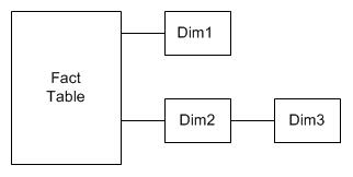
Figure 1. A Reference Dimension connects to the fact table through another dimension
The dimension that connects a reference dimension to the fact table is called 'Intermediate Dimension'. Dim2 in Figure 1 above is an intermediate dimension. The purpose of creating a reference dimension is to expand an attribute in the intermediate dimension so that we can analyze using many attributes in the reference dimension. For example, suppose we have a product dimension table that has a release date column, as shown in Figure 2 below. This column indicates when the product was released into the market. We also have a date dimension table, which has date, month and year columns. Using the date dimension as a reference dimension, we can analyse the release date attribute by year, month and date attributes.
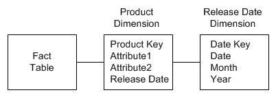
Figure 2. Expanding the Release Date attribute into year, month and date attributes using a reference date dimension
As with everything else, we need to understand the advantages and disadvantages (both sides), and the alternatives. To expand a single date attribute into several date attributes (such as year, month, day, etc), we have 2 options:
- Option 1. Do it in the original dimension
- Option 2. Using a reference date dimension
To do option 1, we need to create Release Year, Release Month and Release Date attributes on the Product dimension. We can create these attributes by modifying the SQL SELECT statement on the Data Source View (DSV). For example, rather than selecting only 1 column like this:SELECT ...,Release_Date,... FROM Dim_Product
we select 3 columns like this:SELECT ...,left(convert(varchar, Release_Date, 20), 10) as Release_Date,
left(convert(varchar, Release_Date, 20), 7) as Release_Month,
datename(yy, Release_Date) as Release_Year,...
FROM Dim_Product
To do option 2, on the cube's Dimension Usage tab we link the Release Date Key attribute on the Product dimension to the Date dimension, as shown in Figure 3 below.
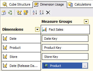
Figure 3. Setting up a Reference Dimension on the Dimensional Usage tab
On option 1 above, the 3 attributes of Release Date will appear under Product Dimension, and only contain the values that exist in the Product dimension's Release Date column. For example, if the Product dimension table does not contain any row with Release Date in January 2001 then the Release Month attribute will not have 'January 2001' member.
On option 2 above, we will have a new dimension called Release Date dimension. This dimension will have the complete set of dates, months and years. There are no missing members like in option 1.
So there are 2 advantages of using a reference dimension:
- We can derive other attributes from a single attribute
- We have complete set of members
There is another advantage of using a reference dimension: consistency of attributes.
Let's say that in the product dimension we have Release Date and Expiry Date. And in the customer dimension we have Registered Date and Leaving Date. For each of these 4 date attributes we want to analyze by: year, quarter, month, week and date. By creating 4 reference dimensions from the same date dimension, we will have a consistent set of attributes, i.e. all 4 dimensions will have the same 5 attributes.
The disadvantage of using a reference dimension is that we can potentially have many additional date dimensions. In the case of Release Date, Expiry Date, Registered Date and Leaving Date that I mentioned in the previous paragraph, we will have 4 additional date dimensions. Having too many date dimensions could potentially lower the cube's user friendliness. When we say 'too many' or 'too much', we need to provide a guide about how much is too much. From my experience 6 date dimensions are too many, where as 3 date dimensions are OK.
So, how do we create a reference date dimension? Let's use the scenario shown in Figure 2 above. First, we need to create a date dimension containing the attributes that we need (year, month, date) attributes and the date key. Then, we add this date dimension to the cube and call it 'Release Date', as shown in Figure 3 above. Then, on the cell where the Release Date dimension intersect with the measure group, we click on the ... button and define the relationship as shown in Figure 4 below:
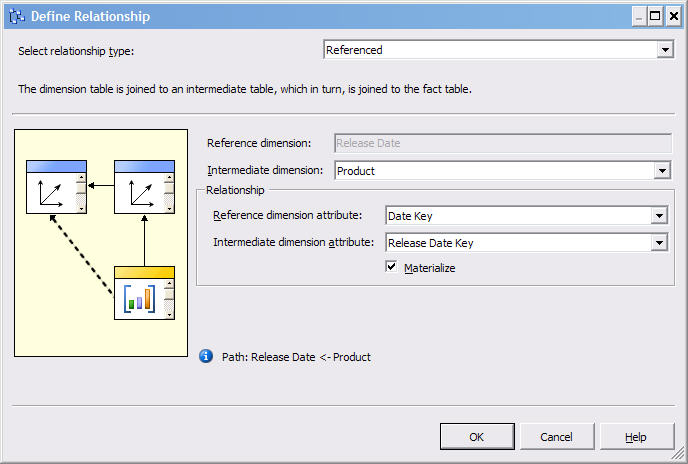
Figure 4. The referenced relationship on Release Date dimension
One of the major considerations when creating a reference date dimension is the date key. Please refer to figure 1 again. The intermediate dimension usually has a date attribute with date type datetime (such as 2009-01-15 00:00:00.000) or varchar (such as '2009-01-15'). Or, in SQL Server 2008, date data type. Where as the reference date dimension may have surrogate key of data type integer (0, 1, 2, 3, ...). So how do we link them if they have different data types?
There are 3 ways:
- Change both of them to surrogate key, e.g. 0, 1, 2, 3, ...
- Change both of them to datetime, e.g. '2009-01-15 00:00:00.000'
- Change both of them to smart date key, e.g. 20081130
Option 1. The advantage of using surrogate key is consistency, i.e. all the dimension keys in the data warehouse are surrogate keys (meaningless incremental integer) and the reference date dimension is no exception. The disadvantages are slightly longer development time and slightly longer cube processing time. This is because we need to lookup the surrogate key. In the case shown in Figure 2, to change the release date column on the product dimension table to release date key, we need to join the table with the date dimension table to get the surrogate key. This is done on the product dimension named query on the data source view (DSV).
Option 2. Using datetime data type as the date key is beneficial when the original date attribute is already in datetime data type. In the case shown in Figure 2, if the release date column on the product dimension is already in datetime data type, we don't need to change anything on the product dimension named query. Every date dimension table has a date column with the datetime data type, so it is straight forward to create a named query that retrieves that column as the primary key.
Option 3. If there is a consensus that through out the data warehouse, all date dimensions use smart date key, then for consistency we need to use smart date key for reference date dimension. I explained the advantages of using smart date key in SSAS in section 3 of this article.
Questions that are quite often asked with regards to reference date dimensions are:
- For the date key, which of the above 3 options is the best one?
It depends on your situation. I have explained the considerations above. Everything else being equal I prefer option 3 provided that a) the SSAS measure groups are partitioned based on date key, and b) the relational fact tables are physically partitioned based on date key. If the date key is not used for partitioning, I prefer to use surrogate key (option 1).
- Is reference dimension not snowflaking? If so, is it bad?
Yes it is snowflaking. On the relational data warehousing, I always prefer star schema than snowflake, but in this case (only on SSAS) reference dimension has its advantages, i.e. ability to analyze by many date attributes and providing a complete set of members. So reference date dimension is good, as long as it's not too much (see the disadvantage of having too many reference date dimensions that I described earlier).
- What is "materialize" in Figure 4? Do we need to use it?
Materialize means that the attributes of the reference dimension (Dim3 in Figure 1) are physically stored in the intermediary dimension (Dim2 in Figure 1), thus improving query performance. Yes, use it by all means. The disadvantage (there are always 2 sides of a coin and we need to see both sides before deciding) is slightly more cube processing time. In the case of reference date dimensions the additional processing time is minimal because they only have tens of thousands members (18,262 members for 50 years). When we say "minimal" or "low" we need to clarify "how low is low". In my experience the additional cube processing time for a materialized reference date dimension is under a second.
2. Server Date Dimension
Server date dimension is a date dimension that is generated by SSAS and stored internally within SSAS. Unlike a normal date dimension, a server date dimension is not created from a physical date dimension table in the data warehouse. In SSAS, server date dimension is also known as 'server time dimension'. I prefer to differentiate 'time dimensions' i.e. hours, minutes, seconds, from 'date dimensions' i.e. year, quarter, month, week, date, so in this article I will use the term 'server date dimension'.
The benefit of using server dimension is that we can have date functionalities without having a physical date dimension table. Practically this usually happens on situations where we don't have access to create a date dimension table in the database or because we don't want to. For example the database may be part of an off-the-shelf application. Or perhaps the database (from which we build the cube) is an Online Transaction Processing (OLTP) database, not a data warehouse. Yes, cubes are also created from 3rd normal form databases such as Operational Data Store (ODS) and OLTP, not only from denormalized, dimensional data warehouse databases.
The other benefit of having a server date dimension is that we can have various attributes and hierarchies without having to create and populate them. For example: manufacturing calendar, fiscal calendar, ISO 8601 calendar and reporting/marketing calendar. Let's briefly go through what they are.
- A regular calendar consists of 12 months and 52 weeks, starts on 1st January.
- A fiscal calendar consists of 12 months and 52 weeks, can start on any date.
- A reporting/marketing calendar consists of 4 quarters with 3 months each. The number of weeks in each of these 3 months can be 4 weeks in the 1st month, 4 weeks in 2nd month, 5 weeks in 3rd month (445 for short), or 454, or 544.
- A manufacturing calendar consists of 3 quarters with 3 periods each and 1 quarter with 4 periods. Each period consists of 4 weeks. There are 13 periods and 52 weeks in a year.
- An ISO 8601 calendar consists of 52 weeks with no months or periods.
The disadvantage of having a server date dimension is inflexibility, i.e. we can't add other attributes, such as special date flag, end of month flag, bank holiday flag, promotion period indicator, etc. We can't change the format in server date dimension. For example, in the fiscal calendar, the year, quarter, month and date attributes are shown in Figure 5 (I use Excel 2007 here to browse the cube). We can't change the year to 'FY 2009', or the month to 'Jan 09', or the date to '1/24/2009'.

Figure 5. Attribute names in server date dimension fiscal calendar
To build a server date dimension, right click on Dimensions on Solution Explorer and choose new dimension, click on Next, choose 'Generate a time table on the server', click on Next, specify the first and last calendar days, the first day of the week, the time periods and the language for member names, as shown in Figure 6 below.
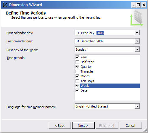
Figure 6. Specifying time periods
Click on Next, choose which calendars you want to create, and specify their details such as 'Start week and month', 'Week by month pattern' and 'Quarter with extra periods', as shown in Figure 7 below.
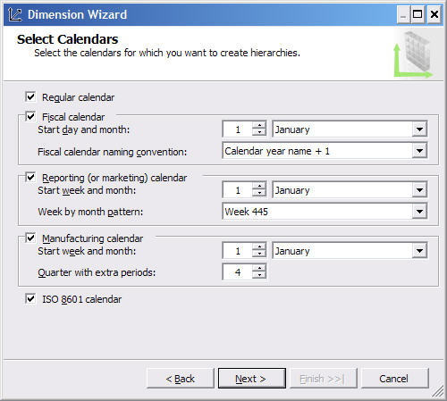
Figure 7. Specifying the calendars and their details
Click on Next, give a name for the date dimension and click on Finish.
3. Smart Date Key
As Ralph Kimball and his group consistently suggested for many years, in dimensional data warehousing the primary keys of dimension tables should be surrogate keys. Surrogate keys means a meaningless sequential integer (e.g. 0, 1, 2, 3, …). I agree with this opinion.
There are 3 main advantages of using surrogate keys:
- To make the data warehouse more flexible to cope with changes in natural key
- To enable the data warehouse to capture history using Slowly Changing Dimension type 2
- To enable the data warehouse to deal with 'unknown', 'not applicable' and 'late arriving' dimension rows
An additional advantage of using surrogate key is query performance (because the joins are on single column integer primary keys).
The alternatives to surrogate keys are using natural keys, or using smart keys. Natural keys are the primary keys of the tables in the source systems. For customer dimension, the natural key is customer ID. For account dimension, the natural key is account number. Date dimension does not have a natural key as there is no source table for it. Even though it doesn't have a source table, we can say that the natural key of a date dimension is the date in date or datetime data type, such as '2009-01-15 00:00:00.000' in SQL Server 2005 (and 2000) datetime data type, or '2009-01-15' in SQL Server 2008 date data type.
Smart key is an integer or character primary key that has a meaning. Each character in the key indicates something. Smart keys are often in the form of concatenation of several items. For product dimension, an example of smart key is Category (2 chars) + Year Launch (YY) + Sequence (3 digits) + Suffix (2 chars), e.g. HC08305FG. For trip (journey) dimension, a possible smart key is Destination-Origin-DepartureDate-Sequence, e.g. HPC-HAC-090115-01. For gas pump (in a gas station), a possible smart key is StationNumber-PumpNumber, e.g. 506-03 (similar technique is applicable for checkout/till dimension in supermarkets). In the case of date dimension, a popular smart key is is YYYYMMDD in integer data type, e.g. 20090115 for January 15th 2009
For relational data warehousing, using surrogate keys is better than using natural keys or smart keys. For date dimension in SSAS (and this is only applicable for date dimension - it's not applicable for any other dimensions), there are 2 advantages of using smart date keys:
- Easier to use the date dimension as a reference dimension, as we don't need to do a look up to translate the dates in the intermediate dimension into the keys.
- Easier to partition the measure group based on the date. To partition a measure group in SSAS, we need to specify a query for each partition. The query is the same for all partitions, except that in the where clause we have an additional condition for partitioning. If we have smart date keys on the fact table, we can use it for this partitioning condition on the where clause. For example, if we allocate each partition to cover a quarter, the additional partitioning condition can be: "where transaction_date_key between 20090101 and 20090331".
How about unknown dates? Unknown dates is handled using unknown member. This is another advantage of using smart date key: unknown dates are not mapped to 01/01/1900, but mapped to the unknown member of the date dimension. This way, in the cube we won't have an awkward year such as 1900, which originated from the unknown row.
4. From Date and To Date
Sometimes, the fact table from which we build the cube from is not transactional. It may contain the balance instead, like this fact_account_balance table:
| Snapshot Month Key | Account Key | Other Dim Keys | Account Balance |
| 200809 | 1 | ... | 120 |
| 200809 | 2 | ... | 750 |
| 200810 | 1 | ... | 120 |
| 200810 | 2 | ... | 880 |
| 200811 | 1 | ... | 300 |
| 200811 | 2 | ... | 880 |
Table 1. Account Balance fact table
In this case, let's assume that the Snapshot Month dimension and Account dimension are like these:
| Snapshot Month Key | Snapshot Month |
| 200809 | September 2008 |
| 200810 | October 2008 |
| 200811 | November 2008 |
Table 2. Snapshot Month dimension table (or view)
| Account Key | Account Number |
| 1 | 10001 |
| 2 | 10002 |
| 3 | 10003 |
Table 3. Account dimension table
The above fact table contains the snapshot of the balance of each account every month. So, accordingly, we build a cube showing the balance of each account for every snapshot month.
If the users want to know the transaction amount between two particular months, we will need to create a calculated measure that calculates the difference, like this:([Snapshot Month].[Snapshot Month].&[200811],[Measures].[Balance])-
([Snapshot Month].[Snapshot Month].&[200809],[Measures].[Balance])
But the problem is, we don't know the value of the two months that the users want until run time. For this situation we can create 2 month dimensions that the user can select. Let's call them 'Month From' and 'Month To'.
The Month From and Month To dimensions are created from the Snapshot Month table (or view). Add both Month From and Month To dimensions to the cube. On the Dimension Usage tab of the cube, do not connect them to the measure group. Leave the Relation Type dropdown list to 'No Relationship', as shown in Figure 8 below.
This way, users will be able to select a member of Month From and Month To dimension, without affecting any measures.
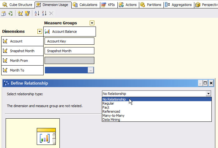
Figure 8. Configuring a dimension for user selection
Then we can create a calculated measure that calculates the difference of balance between Month From and Month To, like this:(StrToMember("[Snapshot Month].[Snapshot Month].&" +
Right(MemberToStr([Month To].[Month To].CurrentMember),8)),
[Measures].[Account Balance])-
(StrToMember("[Snapshot Month].[Snapshot Month].&" +
Right(MemberToStr([Month From].[Month From].CurrentMember),8)),
[Measures].[Account Balance])
The "right(...,8)" function varies depending on the format of the Month From and Month To dimension. The above MDX assumes that the format is [200809] so the MemberToStr function returns "[Month From].[Month From].&[200809]", hence we take the right most 8 characters.
To get the difference of balance between two particular months, the users can select a member on the Month From and Month To dimensions on the slicer axis, put Account Number on the row and put the calculated measure (called Changed Amount) on the column, as shown on Figure 9 below.
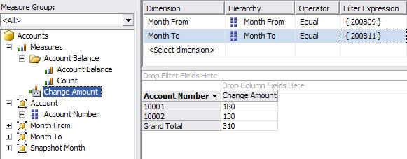
Figure 9. Calculated measure using Month From and Month To dimensions
Or if we use Excel 2007:
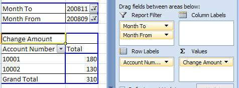
Figure 10. Selecting Month From and Month To dimensions using Excel
And on ProClarity it looks like this:
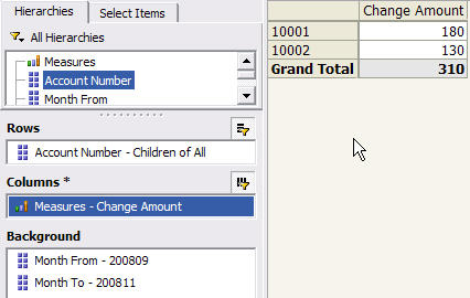
Figure 11. Selecting Month From and Month To dimensions using ProClarity
The above method provides a way to capture user input at run time, i.e. using a date dimension that is not connected to any measure groups. This dimension is used in a calculated measure to select the real date dimension.
5. Other topics about date dimension in SSAS
Among other topics about date dimension in SSAS, by far MDX date functions are the most frequently asked. So in this section, in a limited space, I will try to cover:
- Today's date
- Total until this month
- Year to date
- Month to date
- Last non empty
To get today's date, we can use Now() function. For example, to specify a member of the month attribute with key = "2009-01":Members("[Date Dim].[Month].&[" + Format(Now(), "yyyy-MM") + "]")
To specify a calculated measure that totals a measure from a particular month until this month, we can use "sum((member1:member2),measure)". For example, to create calculated measure [Total To This Month] that sums up Amount measure from April 2008 until this month:with member [Measures].[Total To This Month] as
'sum(([Date Dim].[Month].&[2008-04]:
Members("[Date Dim].[Month].&[" + Format(Now(), "yyyy-MM") + "]")
),[Measures].[Amount]
)'
select [Measures].[Total To This Month] on columns,
[Dim2].[Attribute1].[All].Children on rows
from [Cube]
Note: we can use "aggregate" instead of "sum" and "StrToMember" instead of "Members".
To specify a calculate measure that totals a measure from the beginning of the year until today (year to date), we can use YTD function. For example, to create calculated measure [YTD Amount] that sums up Amount measure from 1st Jan this year until today:with member [Measures].[YTD Amount] as
'sum(YTD(StrToMember("[Date Dim].[Date].&["+Format(Now(), "yyyy-MM-dd")+"]")),[Measures].[Amount])'
select [Measures].[YTD Amount] on columns,
non empty {[Dim2].[Attribute1].[All].Children} on rows
from [Cube]
YTD(x) returns members from the same level as x, from the first member until x, in the same year. For example, if x is 5th May 2008 then YTD(x) is 1st Jan 2008 to 5th May 2008. If we don't specify x, SSAS assumes that x is the current member of date dimension (the dimension with dimension type = Time).
To specify a calculated measure that totals a measure from the beginning of the month until today, we can use PeriodsToDate function. For example,with member [Measures].[MTD Amount] as
'sum(PeriodsToDate([Date].[Month],
StrToMember("[Date Dim].[Date].&["+Format(Now(), "yyyy-MM-dd")+"]")
),[Measures].[Amount])'
select [Measures].[MTD Amount] on columns,
non empty {[Dim2].[Attribute1].[All].Children} on rows
from [Cube]
PeriodsToDate(p,x) returns members from the same level as x, from the first member until x, in period p. For example, if p is Month and x is 5th May 2008, then PeriodsToDate returns the dates from 1 to 5 May 2008. If p is Year and x is August 2008, then PeriodsToDate returns the months from January 2008 to August 2008.
To select the latest date that contains data we can use Tail function:select Tail(NonEmpty([Date Dim].[Date].Members)).item(0) on columns
from [Cube]
Tail returns a set; to get a member out of the set we can use Item function. To select the latest month that contains data, we can change [Date] in the query above with [Month].
The above query examines the default measure. To examine measures other than the default measure, we can replace "NonEmpty" with "NonEmptyCrossJoin", like this:select tail(NonEmptyCrossJoin([Date Dim].[Month].Members * [Measures].[Amount])).item(0).item(0) on columns
from [Cube]
In the above query we use "item(0)" twice because the NonEmptyCrossJoin returns 2 dimensional tuple. The first item(0) returns the measure. The 2nd item(0) returns the month.
Vidas Matelis and
Thomas Ivarsson, two renown experts in SSAS,
provide a handy page
that shows how date-related MDX functions are practically used. It contains useful things like:
list of months up to a specified month, ordering date dimension members in descending order and
getting the first day of the last month in the cube.
So, together with the first part, in this article we have discussed: role play date dimension,
multiple named queries, unknown member, date hierarchies, reference date dimension, server date dimension,
smart date key, capturing user input for calculated measure, and MDX date functions.
I hope that you find this article useful. Date dimension is the most frequently used dimension
in data warehousing, hence it is likely that we will come across date dimension
(and the subjects we discussed above) when building cubes in SSAS. Thank you for reading.
Vincent Rainardi
Author of Building a Data Warehouse With Examples on SQL Server
January 2009


