Microsoft Fabric has OneLake Storage at the center of all services. This storage is based upon existing Azure Data Lake Storage and can be accessed with tools that you are familiar with. Since the invention of computers, many different file formats have been created. Understanding the pros and cons of each file type is important.
Business Problem
Our manager has asked us to understand when to use the following file formats: AVRO, CSV, DELTA, JSON, ORC, PARQUET, and TEXT.
Technical Solution
The preferred format for files in the OneLake is the delta lake tables. However, the OneLake is just a storage account and storage container. Thus, any type of data file can be uploaded to the lake or downloaded from the OneLake. Certain file formats are aligned to how the data is extracted and loaded in the data lake. For instance, REST API calls typically return a JSON payload. Thus, the raw folder might contain JSON data files. However, the DELTA file format is preferred in higher-quality zones.
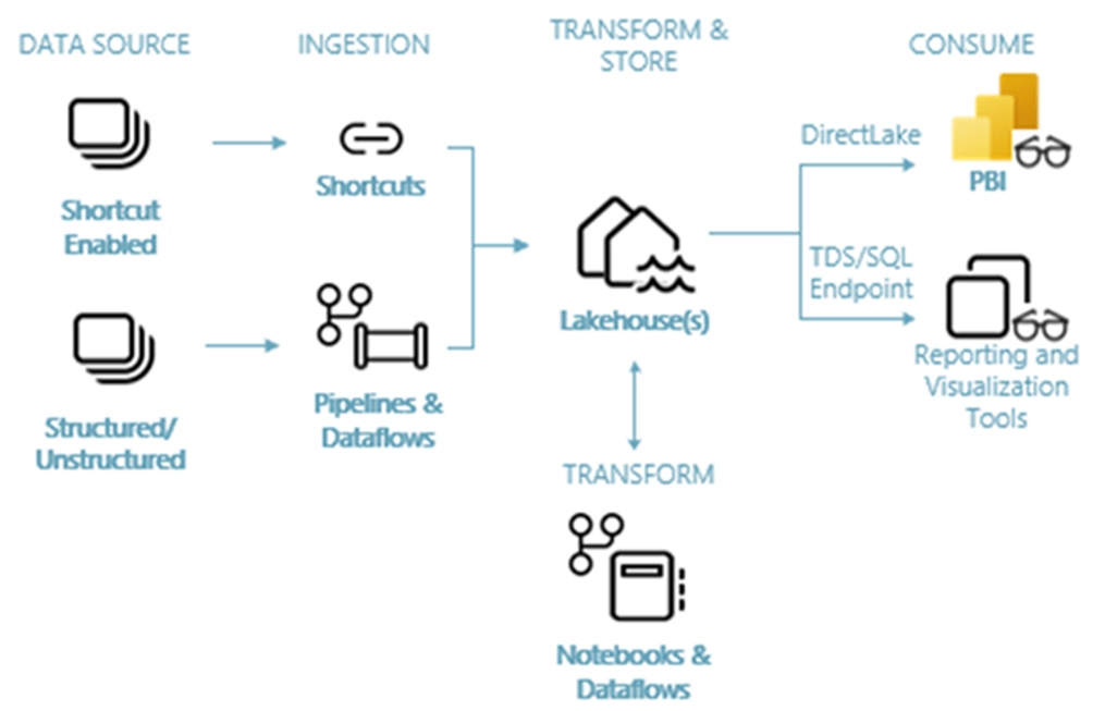
The above image shows how data can get into the OneLake for use with the Lakehouse using shortcuts, pipelines, or dataflows. In prior articles, the author has shown that other tools like Azure Storage Explorer and/or PowerShell can be used to load data into OneLake.
The following topics will be reviewed by the author using Spark notebooks within Microsoft Fabric.
- Review the properties of different file formats
- Transform a CSV file into different formats
- Create managed and/or unmanaged tables
- Summarize data using different tables
Spark Notebooks and Data Files
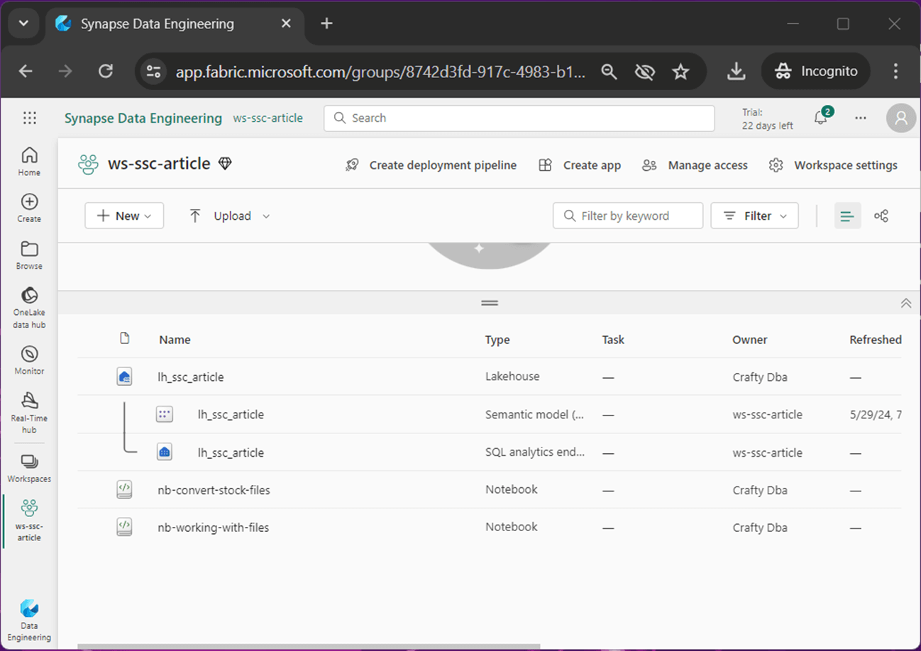
The image below shows a workspace named ws-ssc-article which contains a lakehouse named lh_ssc_article. This Spark engine will provide computing power for the two notebooks. The two notebooks have the following purposes: nb-convert-stock-files transforms AMZN stock data into various file formats and nb-working-with-files demonstrates how to create managed and unmanaged tables. Please note the two notebooks are provided in the Resources sections below.
The image below shows the OneLake storage associated with the Lakehouse. We can see that the stock data has been saved in 6 different formats. A typical use of the TEXT file format is to examine click data from a website. Compressed text data from Nasa’s website will be used as an example.
Comma Separated Values (CSV) File Format
The first use of comma-separated values (CSV) as a data format was with IBM Fortran (level H extended) compiler under OS/360 supported in 1972. I considered this format weak since it can be easily broken by adding additional delimiters.
Strong file formats have the following properties.
- Column data types are known ahead of time without scanning the data.
- Data is stored in a binary format for speed and security.
- Files can be compressed and/or partitioned for large datasets.
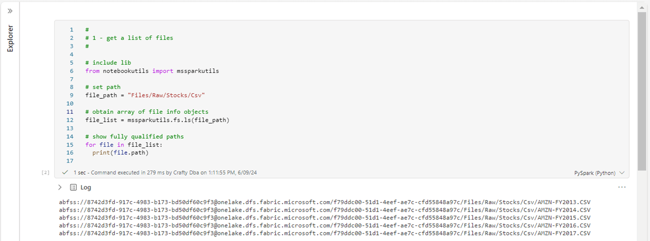
I have manually uploaded five years of Stock data for Amazon. This data will be extracted, transformed, and loaded into different file formats. The mssparkutils library will be used to list the CSV files stored in the folder and retain the fully qualified file paths for future use. Please see image below for details.
Since the source files are in the correct format, we have no more work to do.
Apache Parquet File Format
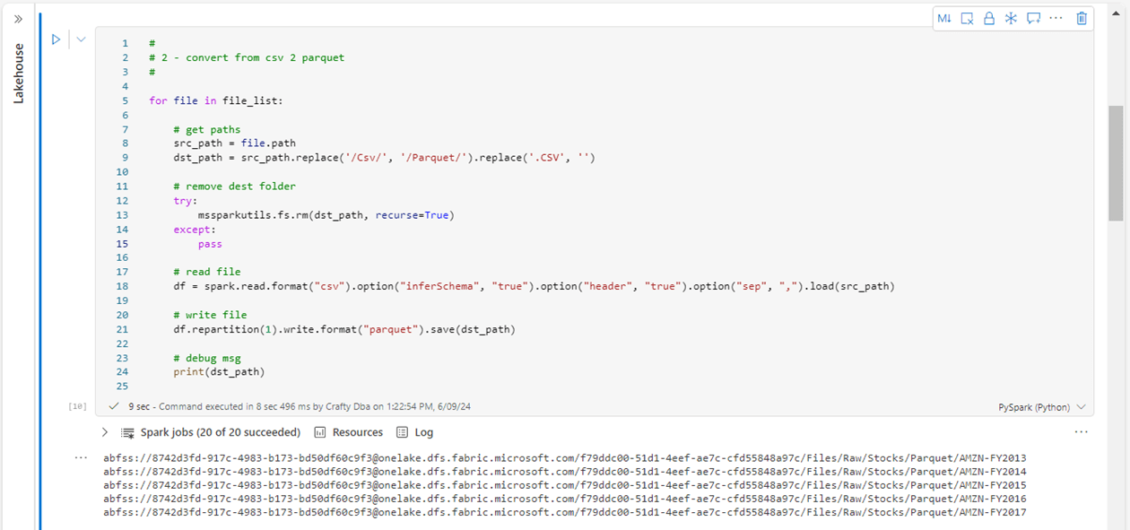
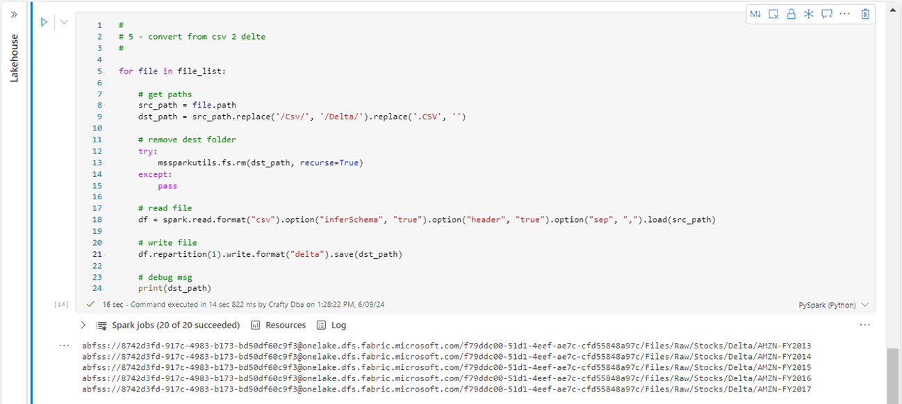
The file_list variable from the previous cell is an array of file objects. For each object, we can read up the source CSV file and write out the contents to a single Parquet file. The image shows the PySpark code. We are using the remove folder command of the mssparkutils library to ensure this process is repeatable. This design pattern will be repeated for each of the file formats.
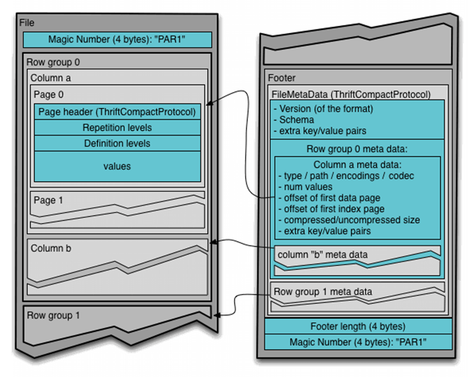
What is the Apache Parquet File format? It is a binary format in which the meta data is separated from the data. Instead of being in a row-based format like CSV, data is stored as column chunks by row. This format lends itself to partitioning as well as compression. Please see the open source website for more information. Parquet is considered a strong file format. Apache Spark has been optimized to work with the parquet file format.
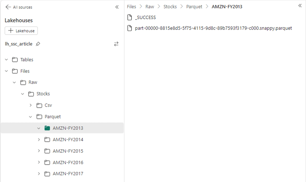
The image below shows a single parquet file that contains stock data for the year 2013. Please note, the repartition command of the Spark Dataframe was used to produce one file (part … c0000.snappy.parquet). The default compression format is snappy. This file format is the foundation of the delta file format that will be explored later.
JavaScript Object Notation File Format
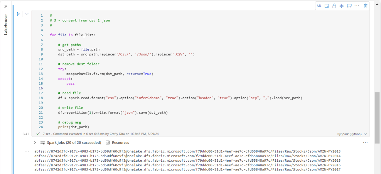
The JSON format grew out of a need for a real-time server-to-browser session communication protocol without using browser plugins. For example, Microsoft supplies the developer with a REST API call to create new Lakehouses in Fabric. Both the input and output to the web service are JSON objects. The image below reads up the CSV file and writes out a JSON file.
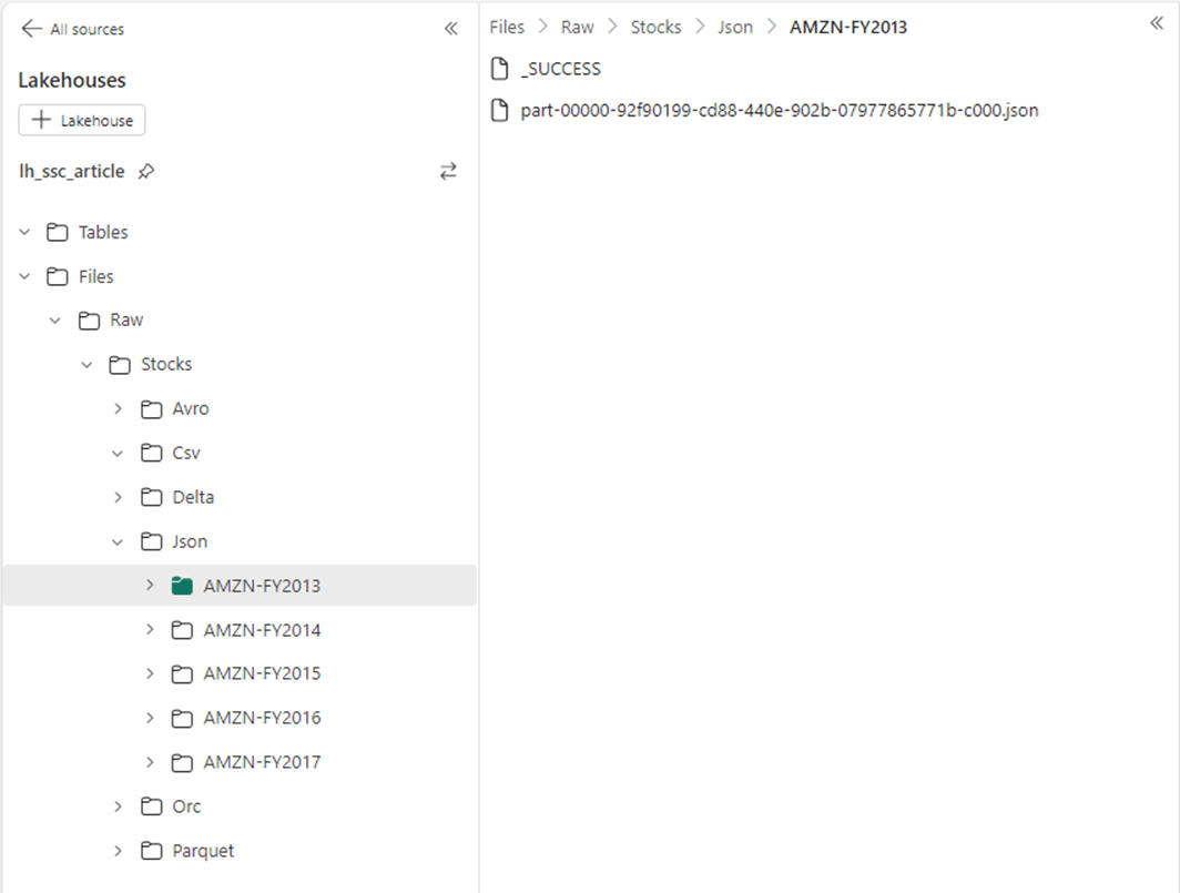
Instead of writing a file, the Apache Spark engine writes a directory. This is required to handle file partitioning. However, if your business consumer needs a single file, save the data using a single partition. Then find the file with the correct extension in the directory and move (rename) the file to a different location. The image below shows a JSON file. JSON is considered a weak file format and is typically large due to repetition of column names.
Apache Avro File Format
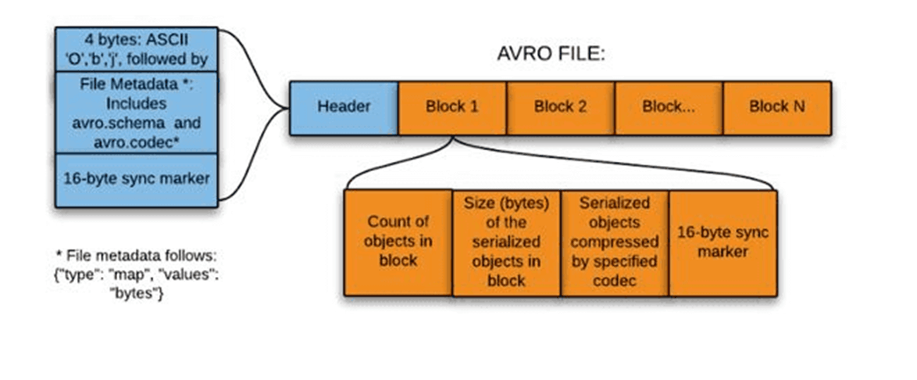
Avro is one of the three formats that came from the Apache foundation. Please see the open-source website for more details. The format was designed to de-serialize data for Remote Procedure Calls (RPC). The metadata for the file is stored in a JSON format while the contents of the file are stored in row fashion. Please see the image below for details.
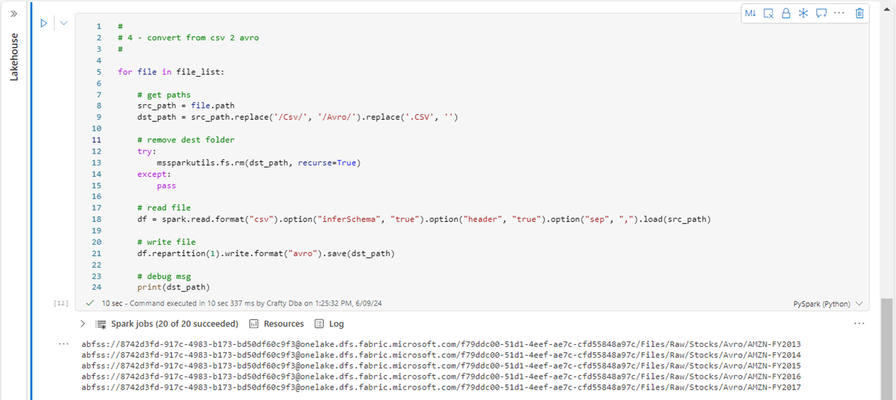
The image below shows the conversion program which reads up a CSV file and writes an Avro file.
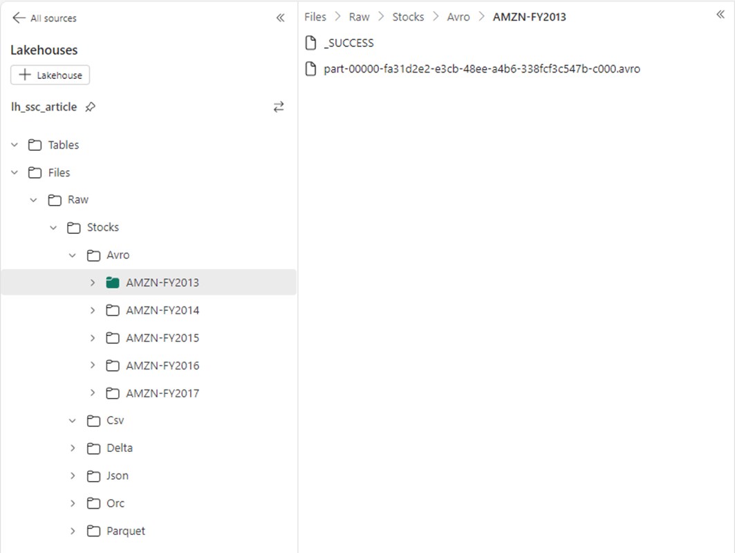
The image below shows five directories, each one containing a single Avro file, were created in the OneLake.
Apache Orc File Format
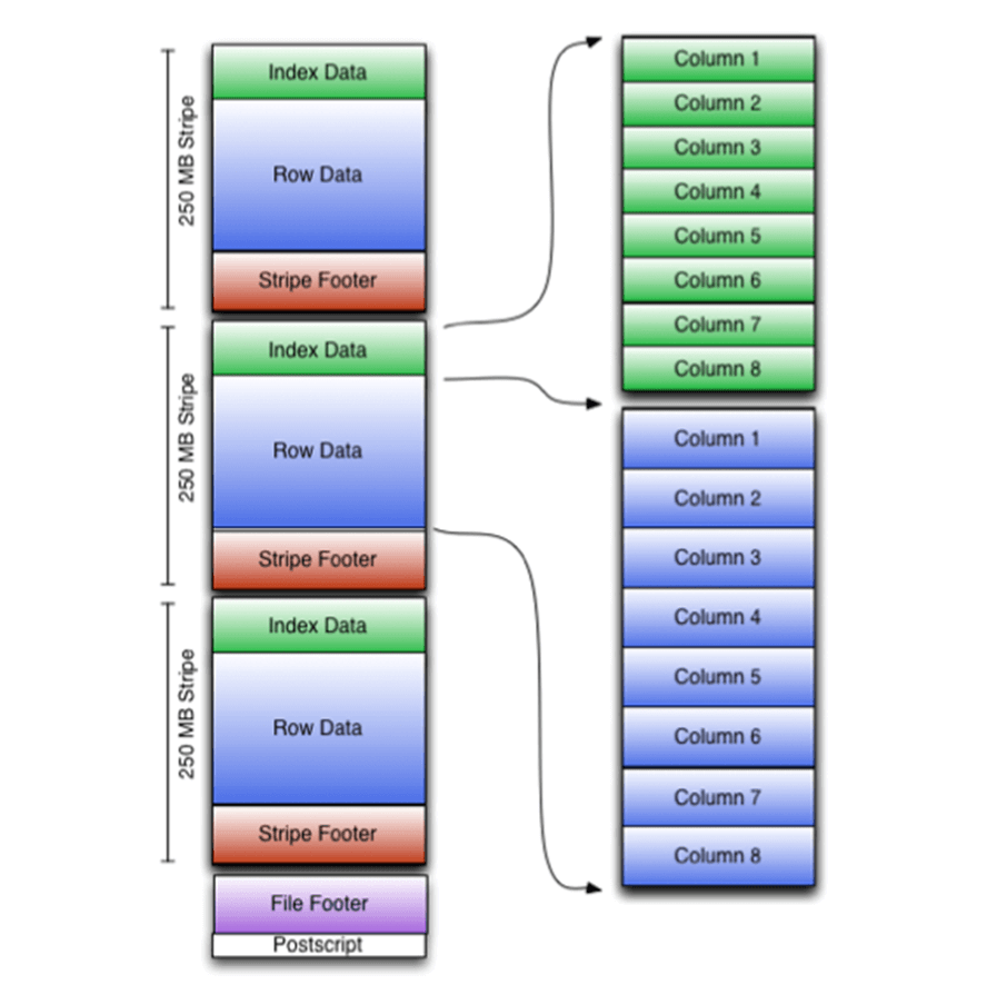
The Apache Optimized Row Columnar (ORC) file format was designed to fix problems with Hadoop’s RC File format. First, the format supports a variety of compression techniques on top of the column store format. Second, projects can be used to read only columns that are required. Third, light weight indexes keep track of min and max values. If pushdown predicates are used, entire sets of rows can be skipped that do not match the WHERE clause. Please see the open source website for details. Please see the image below for an architectural diagram on how data is stored.
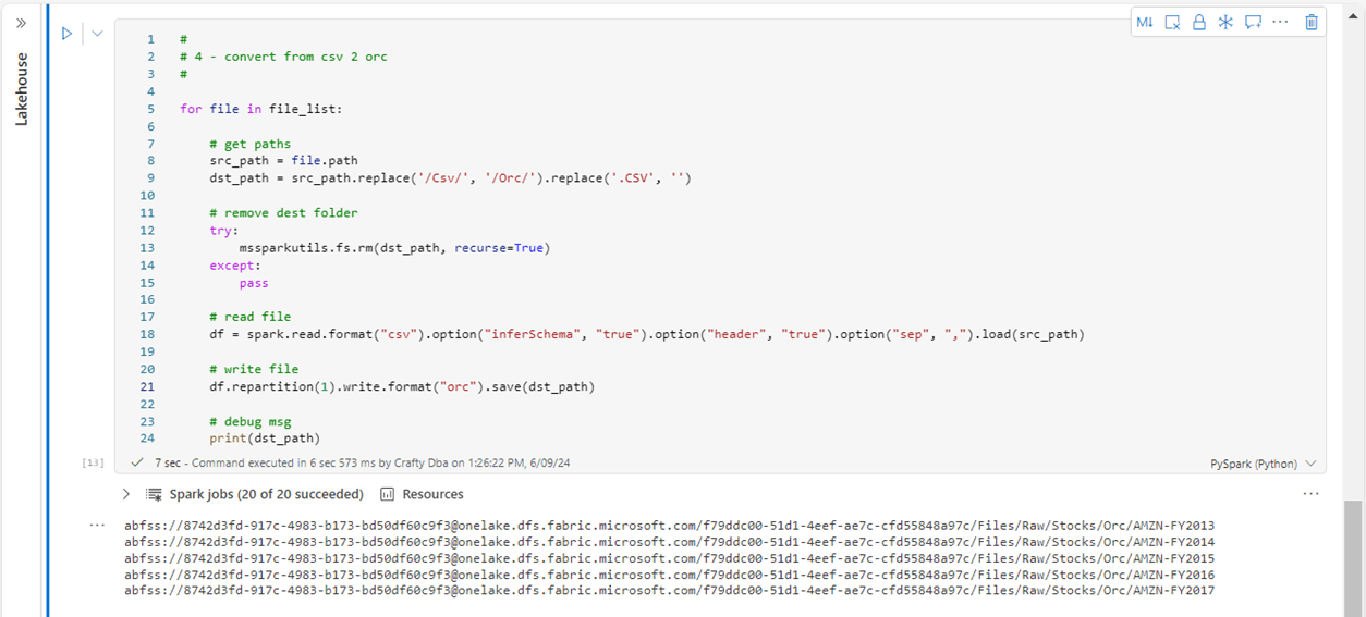
Again, we are going to use a cell in the notebook to convert the Amazon stock data from the CSV to the ORC format.
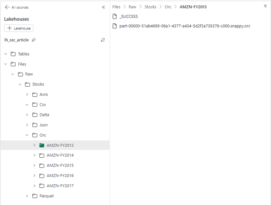
The image below shows the ORC file format that supports compression such as snappy applied after the file is created. In short, ORC is one of the smallest file formats. Apache Hadoop has been optimized to work with the ORC file format.
Delta File Format
Of all the formats we talked about so far, the delta file format is the only one that supports the ACID properties of a database. Thus, if you want to change the contents of a CSV file, one must read in the file, make the appropriate changes, and write out the file. Depending upon the format, the hive table might have to be refreshed after the changes. On the other hand, delta supports inserts, updates, and deletes without any refreshing of the metadata.
Originally, Databricks developed the delta file format. It was given to the open-source community in early 2019. If you have time, please read this article by Mathew Powers. It goes over all the features that DELTA has built on top of PARQUET.
This is the last time we must convert the CSV stock files to another format.
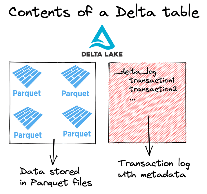
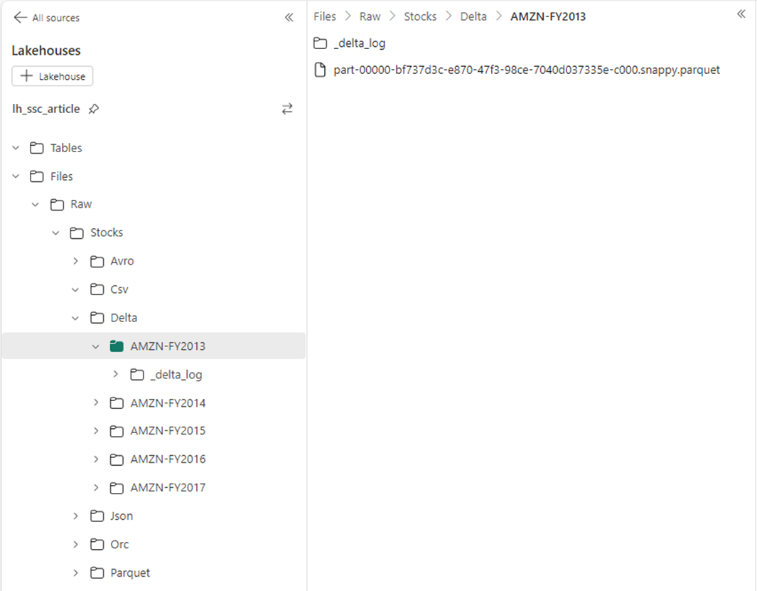
At a quick glance, we can see a parquet file in the folder containing 2013 stock data. The _delta_log folder contains the transaction logs, the metadata file, and the checkpoints. By using this information, the system can support time travel. For instance, what did the table look like yesterday before a bunch of updates occurred.
The total number of trading entries for the Amazon stock between 2013 and 2017 is 1259 rows. This is a very tiny data set since it is stretched over 5 files. I added up the size of all five files given the six file formats. We can see that both AVRO and ORC have very good compression numbers. Both CSV and JSON are ranked last. Since there were no changes to the delta table, the DELTA and PARQUET files are the same size. The differences in file formats will start to show once the volume of data is increased.
Text File Format
The TEXT file format is dependent upon the operating system. For instance, Windows has both a carriage return and line feed to represent the end of line while Linux only has only a line feed. The simplest of these formats is ASCII encoding. There are other code sets such as EBCDIC for the mainframe and UTF-16 to support Unicode. One project I worked on in the past contained Satellite data. This data was stored using two-line element (TLE) formatting.
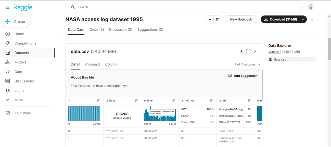
The exploration of web server logs has been of interest to companies for a while. The Kaggle site has a large dataset for Nasa web logs from 1995.
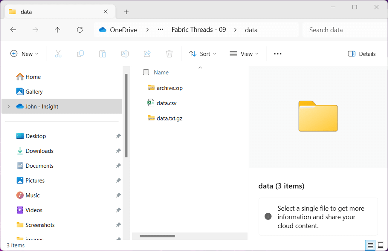
The data from Kaggle comes in a zip file format. Apache Spark supports the gzip file format by default. To make this article smaller, I choose to use the 7-zip application to uncompress to a text file and compress to a gzip file.
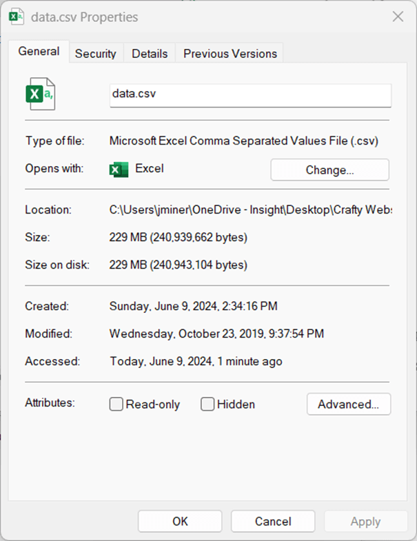
The resulting data file is 229 MB in size.
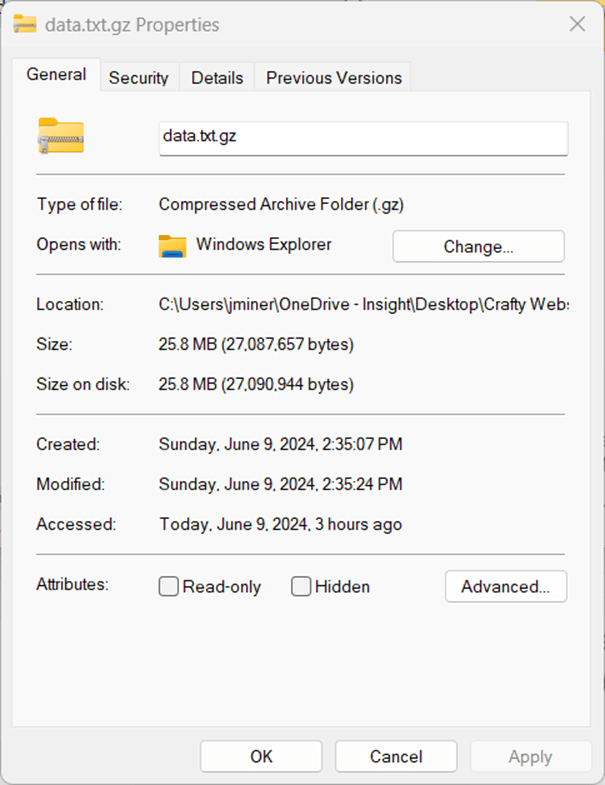
The resulting g-zip file is 25.8 MB in size.
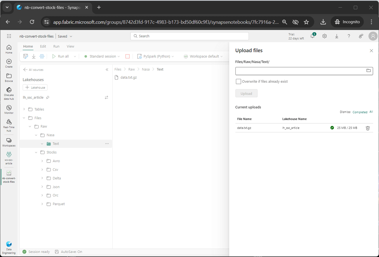
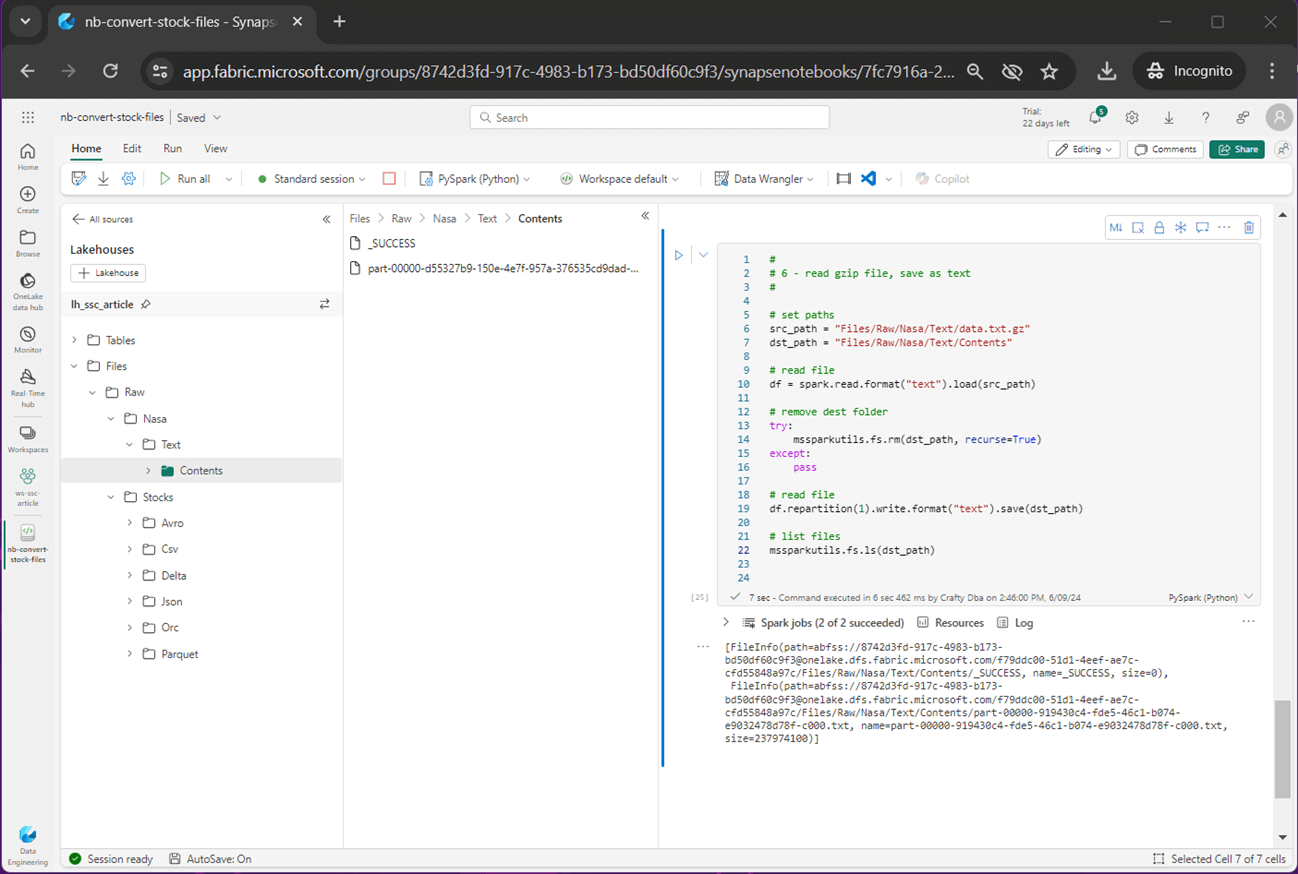
The image below shows the file being uploaded to the folder that is aptly named.
Last, the compressed file is read using PySpark and written out in an uncompressed format. Now that we have examined seven different files formats, it is time to learn about managed and unmanaged hive tables for each format.
Managed vs Unmanaged Hive Tables
Spark SQL supports a shortcut for reading files in a folder. For each of the supported file formats, just use the name of the format followed by directory path inside special tick marks. The drop table statement removes an existing hive entry for the local (managed table). The create table as statement makes a local (managed table) out of the execution results of the select query. This shortcut does not support options such as file header and row delimiter. Thus, we need to rename the columns and remove the header row. Additionally, the date is stored as a string. We can parse out the year and month so that we can create an aggregation query that uses those fields in the result.
--
--  1A - Create managed CSV table
--

-- del
drop table if exists raw_mt_csv_stocks;

-- add
create table if not exists raw_mt_csv_stocks as
    select
        _c0 as _symbol,
        substr(_c1, 7, 4) as _year,
        substr(_c1, 1, 2) as _month,
        _c2 as open,
        _c3 as high,
        _c4 as low,
        _c5 as close,
        _c6 as adjclose,
        _c7 as volume
    from
        csv.`Files/Raw/Stocks/Csv/*`
    where
        _c0 <> 'symbol'
The following spark query returns the total number of rows in the table.
%%sql
select count(*) as total from raw_mt_csv_stocks
We can see that there are only 1259 rows of stock trading data for Amazon over the 5-year period.
The create table using statement always creates an external (unmanaged) table. The code below passes the path, header, and infer schema as optional parameters.
 %%sql

 --
 --  1B - Create unmanaged CSV table
 --

-- del
drop table if exists raw_ut_csv_stocks;

-- add
create table if not exists raw_ut_csv_stocks
using csv
options (path "Files/Raw/Stocks/Csv/*", header "true", inferSchema "true")
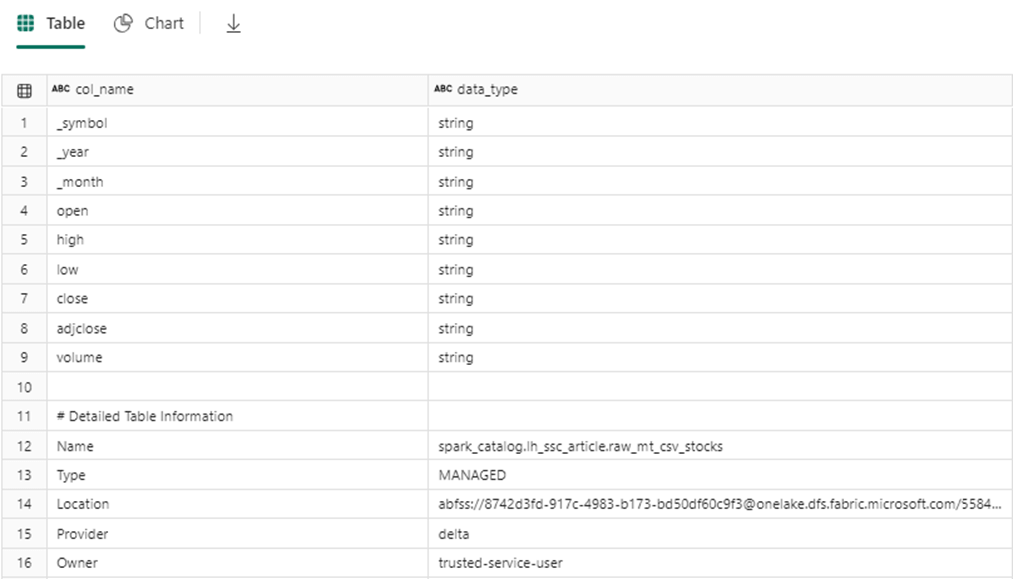
We can use the describe table extended statement to see if a hive table is managed (mt) or unmanaged (ut).
%%sql
--
-- get table info
--
describe table extended raw_ut_csv_stocks
The image below is the output of the describe command executed against the managed table built upon CSV data.
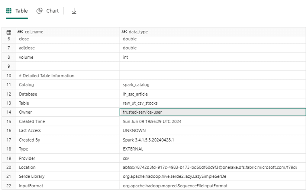
The image below is the output of the describe command executed against the unmanaged table built upon CSV data.
All the other formats can be read in a similar fashion except for the delta file format. One read must be performed per delta file folder. The reason behind this restriction is that all files in the folder must be read to create a consistent view of the data. One way around this problem is to write a Spark SQL query to union all the derived tables together using the shortcut syntax. When using unmanaged tables, a Spark View can be used to union the base hive tables together.
%%sql
 --
 --  6A - Create managed DELTA table
 --

-- del
drop table if exists raw_mt_delta_stocks;

-- add
 create table if not exists raw_mt_delta_stocks as
   select * from delta.`Files/Raw/Stocks/Delta/AMZN-FY2013`
      union
   select * from delta.`Files/Raw/Stocks/Delta/AMZN-FY2014`
      union
   select * from delta.`Files/Raw/Stocks/Delta/AMZN-FY2015`
      union
   select * from delta.`Files/Raw/Stocks/Delta/AMZN-FY2016`
      union
   select * from delta.`Files/Raw/Stocks/Delta/AMZN-FY2017`;
The last step is to aggregate some data.
%%sql

--
-- 1C - aggregate managed CSV data
--

select
    'CSV' as file_type,
    _symbol as trade_symbol,
    _year as trade_year,
    _month as trade_month,
    bround(avg(open), 2) as avg_open,
    bround(avg(close), 2) as avg_close,
    bround(avg(volume), 2) as avg_volume,
    max(high) as max_high,
    min(low) as min_low
from
    raw_mt_csv_stocks
where
    _year = '2016'
group by
    _symbol,
    _year,
    _month
order by
    _year,
    _month
The image below shows the summary information by month for the 2016 year.
I leave it up to the reader to explore the 6 different file formats in relation to managed and unmanaged tables.
Working with Text Files
The text file format allows the developer to parse each line as desired. Spark SQL supports both managed and unmanaged tables. The code below creates a managed table from the data.txt file.
%%sql

 --
 --  7A - Create managed TEXT table
 --

-- del
drop table if exists raw_mt_text_nasa_http;

-- add
 create table if not exists raw_mt_text_nasa_http as
   select * from text.`Files/Raw/Nasa/Text/Contents/*.txt`;
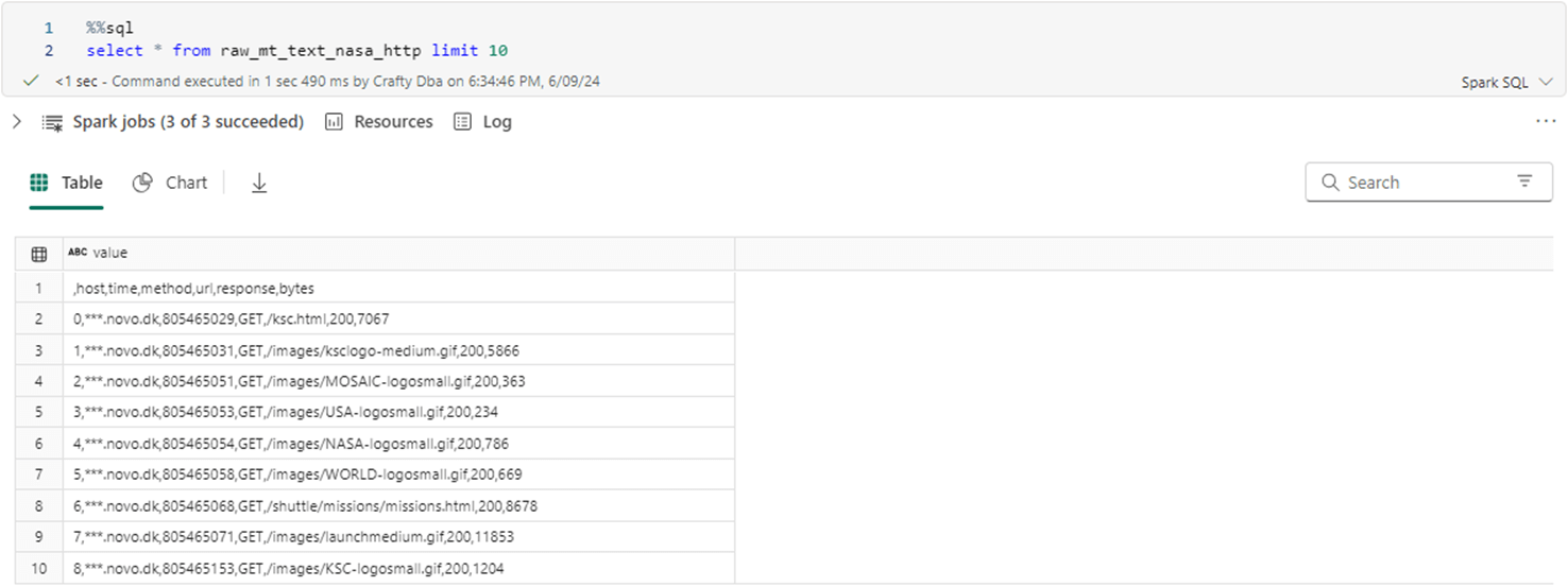
A simple SELECT statement executed on the managed table shows the developer that we could have used the CSV format. However, we would not be able to demonstrate the code pattern to use with text files.
There are two ways to deal with text files. Either search for a pattern in the row and indicate the search result as a boolean flag. Another way is to parse the data into columns of interest. Parsing does not have to use the same delimiter since multiple calls can be made. The split_part function is extremely useful. It returns the nth element after parsing by a delimiter. The row_number function is helpful if we want to eliminate rows by a given value. In our case, we want to remove the header line. The common table expression is used since the filtering on row number is done after the table is calculated.
%%sql
with cte as (
select
    row_number() over (order by 1) as rn,
    split_part(value, ',', 4) as method,
    split_part(value, ',', 5) as url,
    split_part(value, ',', 6) as response
from raw_mt_text_nasa_http
)
select * from cte where rn > 1 and response <> 200 limit 10
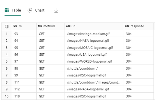
The image below shows the first ten web call failures. Error code 304 means the image has not been modified and the cached version can be used. Use the text file format as a last resort since a lot of coding has to be done to parse the data into usable columns.
Summary
Today, we talked about seven different file formats: AVRO, CSV, DELTA, JSON, ORC, PARQUET, and TEXT. Knowing the properties of each format is important if you want to be a Big Data Engineer. Out of all the formats, the only one that supports insert, update, and delete transactions is DELTA. Many times, data is landed into the raw zone using the native format of the source system. For example, the REST API call to Workday returns information from a custom report. Thus, the JSON format was used to save the file inbound for OneLake.
Both managed and unmanaged tables have their place. Currently, both unmanaged tables and views do not show up in the SQL Endpoint of the Lakehouse. I am hoping the product team fixes this limitation in the future! Just remember, when you drop a managed table, you delete the data from the storage system. I still do a lot of work in Databricks; Therefore, I use unmanaged tables since the storage space of the Azure Databricks service is limited. If you are doing work in Fabric, I suggest you use managed tables in the medallion architecture less the raw zone.
Special text files need special handling. Thus, the text file format can be used to parse these hard to crack files. Going back to the Satellite data that is stored with one row of data on two lines. We can use the row number function to add a line number column to the dataset. Then we can create two common table expressions, one for even rows and one for odd rows. Then we can join the even expressions to odd expressions to obtain the complete row of information.
Enclosed are the two notebooks: one to convert the STOCK data to various file formats and one that can be used to learn about file formats.


