Introduction
In the realm of image generation, Generative Adversarial Networks (GANs) have emerged as powerful tools, capable of creating remarkably realistic visuals. For professionals with decades of experience, witnessing this transformation is akin to seeing the evolution from film to digital photography. This article delves into the fascinating world of GANs, exploring their inner workings and highlighting their potential impact on the field of butterfly image generation, particularly using a dataset of 75 butterfly classes.
Understanding GANs
GANs are a revolutionary approach to image generation, where two neural networks – the generator and the discriminator – engage in a continuous game of "cat and mouse." The generator, the "artist," takes random input and attempts to create new images that resemble real ones. The discriminator, the "art critic," analyses both real and generated images, trying to identify which are fake. This competitive dance between the generator and discriminator drives innovation. As the discriminator gets better at detecting fake images, the generator must learn to create even more realistic ones. This ongoing battle leads to both networks improving, with the generator becoming increasingly adept at generating stunningly realistic images.
The Power of GANs: A Deeper Dive
GANs hold significant potential for various applications, particularly in the realm of butterfly image generation. Their ability to learn and replicate complex patterns can lead to:
- Enhancing Butterfly Conservation Efforts: GANs can generate synthetic images of rare or endangered butterfly species, aiding in conservation efforts by allowing researchers to study their morphology and behaviour without relying on limited real-world data.
- Creating Interactive Educational Experiences: Imagine generating engaging visuals for educational materials or creating interactive virtual environments where users can learn about different butterfly species through realistic simulations.
- Artistic Exploration: GANs can be used as powerful tools for artists, allowing them to explore new artistic expressions and create unique visual interpretations of butterfly imagery.
- Generating Datasets for Machine Learning: GANs can be used to create large datasets of butterfly images for training machine learning models, which can then be applied to tasks like species identification or tracking population dynamics.
A Glimpse into the Architecture
When applying GANs to butterfly image generation, the architecture can be adapted to the specific characteristics of the dataset. The sections below explain how this works.
Generator
The generator network, taking random noise as input, would transform it into an image that closely resembles a butterfly. The generator could be designed with convolutional layers, often with "transpose" operations to increase the image resolution and capture the intricate patterns found in butterfly wings.
# Define the generator network
def build_generator():
    model = keras.Sequential(
        [
            layers.Dense(128 * 28 * 28, use_bias=False, input_shape=(200,)),
            layers.BatchNormalization(),
            layers.LeakyReLU(),
            layers.Reshape((28, 28, 128)),
            layers.Conv2DTranspose(128, kernel_size=3, strides=2, padding="same", use_bias=False),
            layers.BatchNormalization(),
            layers.LeakyReLU(),
            layers.Conv2DTranspose(64, kernel_size=3, strides=2, padding="same", use_bias=False),
            layers.BatchNormalization(),
            layers.LeakyReLU(),
            layers.Conv2DTranspose(32, kernel_size=3, strides=2, padding="same", use_bias=False),
            layers.BatchNormalization(),
            layers.LeakyReLU(),
            layers.Conv2DTranspose(3, kernel_size=3, strides=1, padding="same", activation="tanh"),
        ],
        name="generator",
    )
    return model
Discriminator
The discriminator network would analyze images (both real and generated), trying to classify them as either real butterflies or fakes. It would likely use convolutional layers with down sampling to extract features and identify discrepancies between real and generated images.
The Training Process is a Step-by-Step Process that includes:
- The Artist's Struggle: The generator constantly tries to create images that fool the discriminator.
- The Critic's Guidance: The discriminator gets better at identifying fake images, forcing the generator to improve its skills.
- Continuous Improvement: This iterative process, where the generator learns from the discriminator's feedback, leads to increasingly realistic and beautiful butterfly images.
# Define the discriminator network
def build_discriminator():
    model = keras.Sequential(
        [
            layers.Conv2D(64, kernel_size=3, strides=2, padding="same", input_shape=[224, 224, 3]),
            layers.LeakyReLU(),
            layers.Dropout(0.3),
            layers.Conv2D(128, kernel_size=3, strides=2, padding="same"),
            layers.LeakyReLU(),
            layers.Dropout(0.3),
            layers.Conv2D(256, kernel_size=3, strides=2, padding="same"),
            layers.LeakyReLU(),
            layers.Dropout(0.3),
            layers.Flatten(),
            layers.Dense(1, activation="sigmoid"),
        ],
        name="discriminator",
    )
    return model
Model Instantiation
generator = build_generator() and discriminator = build_discriminator(): These lines create instances of the generator and discriminator models, respectively. The build_generator() and build_discriminator() functions (not shown here) would define the specific architectures of these neural networks, using layers like convolutional layers, dense layers, etc.
# Create instances of generator and discriminator models
# define the specific architectures of these neural networks
generator = build_generator()
discriminator = build_discriminator()
Training Hyper-parameters
We need to define hyper-parameters to control the generation.
- BATCH_SIZE = 16: This defines the number of images that are processed in each training step. A larger batch size can sometimes speed up training, but requires more memory.
- noise_dim = 200: This indicates the dimension of the random noise vectors that are fed to the generator. The generator learns to convert this noise into realistic butterfly images.
- epochs = 100: This defines the total number of training epochs (complete passes through the dataset). More epochs generally lead to better results but require more training time.
# Define hyper-parameters
BATCH_SIZE = 16
noise_dim = 200
epochs = 100
Loss Functions and Optimizers
Here, we need to define the cross entropy which computes the cross-entropy loss between true labels and predicted labels.
Then define the discriminator_loss which calculates the total loss.
# Define the cross-entropy loss function
cross_entropy = tf.keras.losses.BinaryCrossentropy()
# Define the discriminator loss function
def discriminator_loss(real_output, fake_output):
    real_loss = cross_entropy(tf.ones_like(real_output), real_output)
    fake_loss = cross_entropy(tf.zeros_like(fake_output), fake_output)
    total_loss = real_loss + fake_loss
    return total_loss
# Define the generator loss function
def generator_loss(fake_output):
    return cross_entropy(tf.ones_like(fake_output), fake_output)
The Training Loop
Here is the code that trains our generator. The Outer Loop (Epochs) iterates for the specified number of epochs. Each epoch represents a complete pass through the dataset.
The Inner Loop (Batches) iterates over each batch of images in the dataset. This is where the actual training happens.
# Define the training step function
@tf.function
def train_step(images):
    noise = tf.random.normal([BATCH_SIZE, noise_dim])
    with tf.GradientTape() as gen_tape, tf.GradientTape() as disc_tape:
        generated_images = generator(noise, training=True)
        real_output = discriminator(images, training=True)
        fake_output = discriminator(generated_images, training=True)
        gen_loss = generator_loss(fake_output)
        disc_loss = discriminator_loss(real_output, fake_output)
    gradients_of_generator = gen_tape.gradient(gen_loss, generator.trainable_variables)
    gradients_of_discriminator = disc_tape.gradient(disc_loss, discriminator.trainable_variables)
    generator_optimizer.apply_gradients(zip(gradients_of_generator, generator.trainable_variables))
    discriminator_optimizer.apply_gradients(zip(gradients_of_discriminator, discriminator.trainable_variables))
The line with train_step(images) calls the train_step function, which is the core of the GAN training process. This function does the following:
- Generates random noise.
- Passes the noise to the generator to create fake images.
- Passes both real and fake images to the discriminator for classification.
- Calculates the loss for both the generator and the discriminator.
- Updates the weights of both networks using their respective optimizers.
# Train the GAN
for epoch in range(epochs):
    for images in dataset:
        train_step(images)
The last code snippet, Generating and Displaying Images, indicates that, likely every 10 epochs, you might generate a sample of images from the generator and display them using Matplotlib to visualize how the training is progressing.
# Generate and display images
    if (epoch + 1) % 10 == 0:
        noise = tf.random.normal([BATCH_SIZE, noise_dim])
        generated_images = generator(noise, training=False)
        fig, axs = plt.subplots(4, 4, figsize=(8, 8))
        for i in range(4):
            for j in range(4):
                axs.imshow((generated_images.numpy() + 1) / 2)  # Rescale images to [0, 1]
                axs.axis("off")
        plt.show()
Interpretation
- test_image_path = '/content/Image_1.jpg': This line defines the path to the test image you want to use. Make sure this path points to a valid image file in your directory.
- test_image = tf.io.read_file(test_image_path): This reads the image from the specified path as raw bytes.
- test_image = tf.image.decode_jpeg(test_image, channels=3): This decodes the image data (assuming it's in JPEG format) and converts it to a tensor with three color channels (RGB).
- test_image = tf.image.resize(test_image, (224, 224)): This resizes the image to 224x224 pixels, which is likely the input size expected by your trained GAN model.
- test_image = tf.cast(test_image, tf.float32): This converts the image data from integers to floating-point numbers for numerical stability in TensorFlow.
- test_image = (test_image / 127.5) - 1: This normalizes the pixel values of the image to the range [-1, 1], which is a common normalization scheme for GANs.
# Load and preprocess a single test image
test_image_path = '/content/Image_1.jpg'
test_image = tf.io.read_file(test_image_path)
test_image = tf.image.decode_jpeg(test_image, channels=3)
test_image = tf.image.resize(test_image, (224, 224))  # Resize to match the input size of your model
test_image = tf.cast(test_image, tf.float32)
test_image = (test_image / 127.5) - 1  # Normalize to [-1, 1]
Generating a Single Image with the Generator
- test_generated_image(generator, noise_dim): This function generates a single image using the trained generator (generator).
- noise = tf.random.normal([1, noise_dim]): It generates a random noise vector of size [1, noise_dim] (where noise_dim is likely the same value you used during training).
- generated_image = generator(noise, training=False): The generator then takes this noise as input and generates a butterfly image. The training=False argument ensures that the generator is in inference mode (not training).
# Generate a single image using the generator
def test_generated_image(generator, noise_dim):
    noise = tf.random.normal([1, noise_dim])
    generated_image = generator(noise, training=False)
    return generated_image
Visualizing the Results
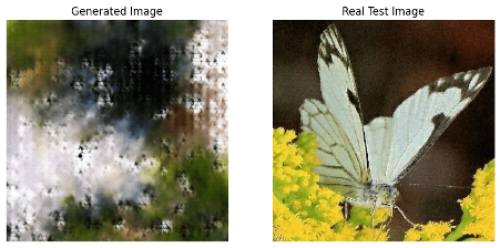
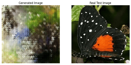
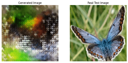
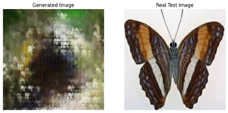
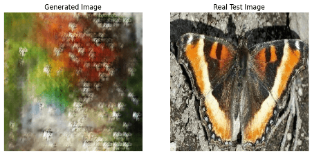
- visualize_single_result(generator, test_image, noise_dim): This function displays the generated image side-by-side with the real test image.
- generated_image = test_generated_image(generator, noise_dim): It calls the test_generated_image function to generate a new image.
- fig, axs = plt.subplots(1, 2, figsize=(10, 5)): It sets up a figure with two subplots (one for the generated image and one for the real image).
- axs[0].imshow(...), axs[1].imshow(...): The generated image and the real test image are displayed in the subplots, with appropriate titles and axes turned off.
# Test the generated image against the single test image
def visualize_single_result(generator, test_image, noise_dim):
    generated_image = test_generated_image(generator, noise_dim)
    fig, axs = plt.subplots(1, 2, figsize=(10, 5))
    # Plot generated image
    axs[0].imshow((generated_image[0].numpy() + 1) / 2)
    axs[0].set_title('Generated Image')
    axs[0].axis("off")
    # Plot real test image
    axs[1].imshow((test_image.numpy() + 1) / 2)
    axs[1].set_title('Real Test Image')
    axs[1].axis("off")
    plt.show()
# Call the function to visualize the result
visualize_single_result(generator, test_image, noise_dim)
Sample output
Conclusion
The journey of teaching a computer to paint realistic butterflies with Generative Adversarial Networks (GANs) has been a captivating exploration of artificial creativity. By observing the dynamic interaction of the generator and discriminator – the artist and critic – we've witnessed the transformative power of this technique.
GANs have demonstrated their potential to generate incredibly lifelike images, blurring the lines between reality and artificial creation. The ability to produce realistic butterfly images opens up a wealth of possibilities in conservation, education, art, and even the advancement of machine learning.
Future Enhancements
While we've made significant strides, there's always room for improvement. Here are some exciting directions to explore:
- Improving Image Quality: We can strive for even more realistic and detailed butterfly images by exploring new GAN architectures, optimizing hyper-parameters, and incorporating more diverse training data.
- Fine-Grained Control: Giving users more control over the image generation process, such as specifying desired wing patterns or colours, would enhance the artistic capabilities of the model.
- Generative Adversarial Networks for Video: Extending GANs to generate videos of butterflies in flight or their interactions with their environment would create captivating and educational content.
- Multi-Modal GANs: Integrating other sensory data, such as sound or touch, into the GAN model could create a more immersive and multi-dimensional experience.


