In our previous article, Identifying Customer Buying Patterns in Power BI—Part 1, we described the customer purchase product frequency. In this article, we will be conducting an advanced analysis in Power BI via a market-based analysis (MBA) technique called basket analysis. Therefore, we will be creating the basket analysis DAX formula. Part 3 of identifying customer buying patterns in Power BI will cover metrics related to the "association rule". The data in this article, Power BI Auto-Detect Relationship Failure, has already been produced.

What is Basket Analysis?

Basket analysis is used mostly for identifying customer buying patterns as a data mining technique. Therefore, to analyze which products customers have bought together, we will be applying the "association rule". Below are the main metrics used in basket analysis to apply the association rule.

Support

It is calculated by dividing the total number of transactions, which includes both item Product 1 and item Product 2—by the total number of transactions made.

Support = (Product 1 + Product 2) ÷ Total Transaction

Support (Items) = (Egg + Bread) ÷ Total Transaction

 Support = 2 ÷ 4 = .5

Confidence

The ratio represents the total number of transactions that contain every item from both (Product 1) and (Product 2) compared to the total number of transactions that contain every item from (Product 1).

Confidence = (Product 1 + Product 2) ÷ Product 1

Confidence (Items) = (Egg + Bread) ÷ Egg

Confidence = (2) ÷ 1 = 2

Lift

It is the ratio of confidence to expected confidence. Expected confidence is the confidence divided by the frequency of Product 2. The Lift tells us how much better a rule is at predicting the result than just assuming the result in the first place. Greater lift values indicate stronger associations.

Lift = [ ((Product 1 + Product 2) ÷ Product 1) / (Product 2 ÷ Total)]

Lift (Items) = ((Egg + Bread) ÷ Egg) / (Bread ÷ Total)

Lift = ((2) ÷ 1) / (1 ÷ 4) = 2/.25 = 8

Creating a Basket Analysis Table in Power BI via DAX

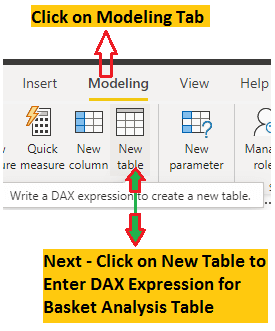
This stage will involve creating a basket analysis table using DAX. Using the sales data, it will generate every pair of products that can be purchased. You will get to the table on the fields tab after clicking the modeling tab and the new table button in the ribbon.

111111

The New Table dialog will appear as shown in the screenshot below.

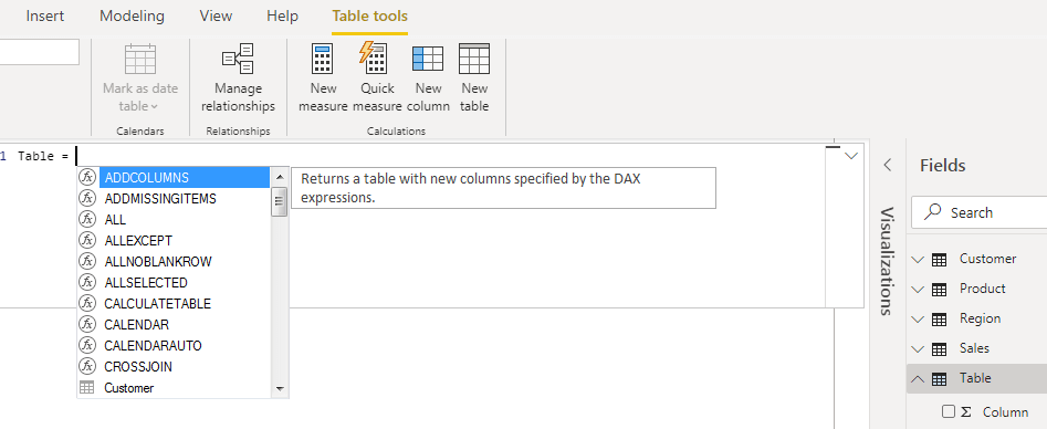
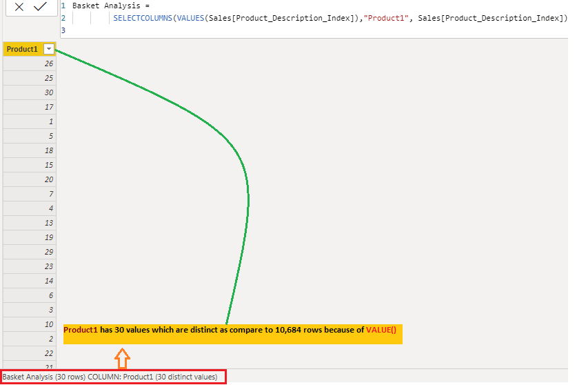
Initially, we will use VALUE() in conjunction with SELECTCOLUMNS() to retrieve the distinct values from the product column. To find out more about VALUE() and SELECTCOLUMNS(), please click the link.

 Basket Analysis = 
SELECTCOLUMNS(VALUES(Sales[Product_Description_Index]),"Product1", Sales[Product_Description_Index])

Here is the output for the above formula.

In the next step, we created a "Product 2" column; similarly, we created a DAX formula for "Product 1" under Basket Analysis. In order to create a second column for "Product 2" within the Basket Analysis DAX formula, we will copy the first formula and replace "Product 1" with "Product 2". Please see the below screenshot as a reference.

Basket Analysis = 
SELECTCOLUMNS(VALUES(Sales[Product_Description_Index]),"Product2", Sales[Product_Description_Index])

Once we get the two columns, Product1 and Product2, we will apply CROSSJOINS(). This will produce all the possible combinations. Hence, we will have 900 rows coming from all the rows in Product 1 (30 rows) multiplied by all the rows from Product 2 (30 rows). This creates a Cartesian product of 900 rows.

Basket Analysis = 
CROSSJOIN(
  SELECTCOLUMNS(VALUES(Sales[Product_Description_Index]),"Product1", Sales[Product_Description_Index]),
  SELECTCOLUMNS(VALUES(Sales[Product_Description_Index]),"Product2", Sales[Product_Description_Index])
          )

Below is the partial output for the above formula, which produces 900 rows due to the CROSSJOINS() between "Product 1" (30 rows) and multiplying all the rows from "Product 2" (30 rows).

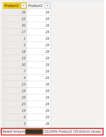
As for the next step in our basket analysis, we want to remove duplicate rows where the values in both Product 1 and Product 2 columns are identical, but only if these duplicates appear consecutively. For instance, in the table above, Product 1 with a value of 29 and Product 2 with a value of 29 have 2 consecutive duplicates.

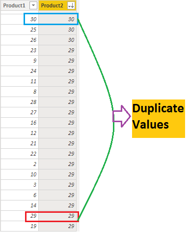
In order to remove duplicates, we will be applying FILTER(). The logic we will apply for FILTER() is that we filter based on Product 1 > Product 2.

Basket Analysis = 
FILTER(
        CROSSJOIN(
   SELECTCOLUMNS(VALUES(Sales[Product_Description_Index]),"Product1", Sales[Product_Description_Index]),
   SELECTCOLUMNS(VALUES(Sales[Product_Description_Index]),"Product2", Sales[Product_Description_Index])
                ), 
       [Product1] > [Product2]
        )

The above query in the image doesn't eliminate entire records, it reduces the number of rows by filtering out duplicate combinations of product descriptions. Instead of 900 rows, it would return 435 rows containing only unique pairings of products in the "Product 1" and "Product 2" columns. So, it identifies all possible unique baskets of two items, rather than grouping together all occurrences of those products.

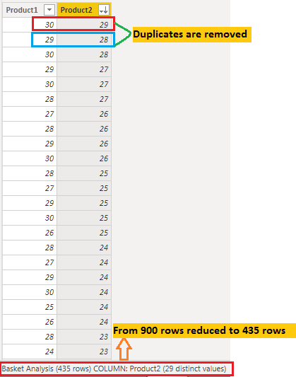
In a final step, we will be creating a new calculated column "Basket", merging both Product1 and Product 2.

Basket = 'Basket Analysis'[Product1] & "-"  & 'Basket Analysis'[Product2]

Below is the output for above formula. ⇑

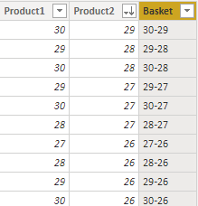
Now, we have all the unique combinations in our basket columns for our 30+ products. It will give us the foundation to calculate the metrics applied in the association rule, which are support, confidence, and list. These metrics will be covered in Part 3.