by Steve Bolton

                Anyone who’s gotten this far in this series of amateur self-tutorials on SQL Server Data Mining (SSDM) is probably capable of using it to unearth some worthwhile nuggets of wisdom in their data. One of the key remaining questions at this step of our rickety stairway is what we can do with the information we’ve mined. The most obvious answer to this would be to act upon the information; we must not lose sight of the fact that our ultimate mission is not to simply dig up truths based on past data for a person or organization, but to enable them to act with greater precision in the present to ensure a better future. Any subject under the sun may an intrinsic worth of its own, but appreciation for anything should not be divorced from its wider uses and implications for everything else beyond it; this is the point at which intellectuals to get lost in Ivory Towers and become irrelevant to the wider world outside their narrow vision. This also happens in the discipline of history, which I have some claim to real expertise in – unlike with SSDM, which I am writing about in order to familiarize myself with the topic better while simultaneously giving SQL Server’s most neglected component some badly needed free press. Sometimes historians get lost in mere antiquarian appreciation for their narrow specialties, while ignoring the more important tasks of helping mankind avoid fulfilling Santayana’s classic warning, “Those who cannot remember the past are condemned to repeat it.” Likewise, as the field of data mining blossoms in the coming decades, it will be critical to keep the giant mass of truths it is capable of unearthing relevant to the goals of the organizations the miners work for. Knowledge is worth something on its own, but it should also be remembered that “Knowledge is power.” Francis Bacon’s famous quip is incomplete, however, because knowledge is only one form of power; as Stephen King once pointed out in typically morbid fashion, it doesn’t do a mechanic whose car jack has slipped much good to truly know that he’s powerless to move the automobile crushing his chest. I suspect this is a fine distinction that will come to the fore as data mining matures. The most critical bottlenecks for organizations in the future, once data mining has become ubiquitous, may be the challenge of acting on it. The poor soul in Stephen King’s example can’t act on his information at all. Many organizations, however, may prove incapable of acting on good data due to other internal faults. Eight centuries ago, St. Thomas Aquinas pointed out that sometimes people prove incapable of doing things they know they ought to do, despite telling themselves to do them; such “defects of command” may well become glaringly evident in the future, as the next bottlenecks in unsuccessful organizations.

                At that point, data mining may already be automated to the point where algorithm processing results mechanically trigger actions by organizations. Some relational databases and data warehouses already have the capability of doing this to a degree, such as automatically sending out new orders to replenish inventories before they are depleted, or triggering a stock trade. Yet in most cases these automated decisions are based on fairly simple functions, not the ultra-, uber-, mega-sophisticated functions that modern data mining algorithms amount to. One day Wall Street firms may rise and fall in a day depending on whether the gigantic data warehouse at the center of an organization can out-mine its competitors and therefore out-trade them, without any human intervention at all since the formulas they’re acting on are too complex to put into human language; this would be a strange twist indeed on the science fiction chestnut of artificial intelligence gone awry. Using some of the scripts I’m going to provide in this post in conjunction with ADO.Net, SQL Server Integration Services (SSIS) and XML for Analysis (XMLA), we could indeed start laying the foundations for such automated processes right now, if need be.  The problem is that data mining is still in its infancy, to the point where it would be quite unwise for any organization to automatically rely on its mining results without prior human review by an actual intelligence. Our next programming task could thus be to build systems that automatically act on data mining results, but for the meantime it is much more prudent for humans to review the results first, then decide on courses of action themselves. That is probably why SSDM, or any other mining software I’m aware of, lacks built-in ways of handling such functionality. Without it, programmers are left with two other tasks they can perform on data they’ve already mined: present it more efficiently so that people can analyze it from a human perspective, or to feed the data back into mining process for further computational analysis. Either way, we’re talking about mining the mining results themselves; the process can be looked at as continuously refining hydrocarbon fuels or cutting diamonds we’ve taken from the ground, until they reach the point where the cost of further refining outweighs further improvements in quality. To perform the latter task, we need some programmatic means of feeding mining results from SSDM back into the mining process. Keep in mind that this is a fairly advanced task; it is obviously much more important to mine data the first time, as the previous posts in this series explained how to do, than to feed them back into the system reiteratively. It is not as advanced or risky as automated action though. That is probably why some limited means to perform the former task are provided in SSDM, but not any out-of-the-box solutions to the latter one.

               Such nascent functionality is included in SSDM in the form of data mining dimensions, which incorporate your mining results into a SQL Server Analysis Services (SSAS) cube. The official documentation carries a caveat that makes all the difference in the world: “If your mining structure is based on an OLAP cube.” The practice data I used throughout this series came strictly from relational data, because I didn’t want to burden DBAs who come from a relational background with the extra step of first importing our data into a cube, then into SSDM. That is why I was unable to add a data mining dimension through the usual means of right-clicking on a mining model and selecting the appropriate menu item, as depicted in Figure 1. I discovered this important limitation after getting back just 34 hits for the Google search terms “’Create Data Mining Dimension’ greyed” (or grayed) – all of which led to the same thread at MSDN with no reply.

Figure 1: Mining Dimension Creation Menu Command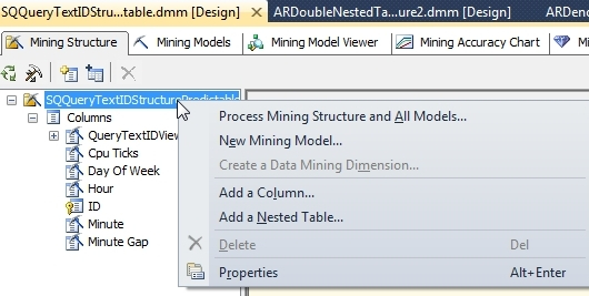

                The rest of the screenshots in this post come from another project I started practicing on a long time ago, which was derived from cube data and therefore left the Create a Data Mining Dimension command enabled. Selecting it brings up the dialog in Figure 2, which performs the same function as the Create mining model dimension checkbox and a Create cube using mining model dimension checkbox on the Completing the Wizard page of the Data Mining Wizard. It’s all fairly self-explanatory.

Figure 2: Mining Dimension Creation Dialog Box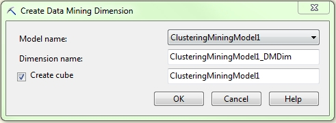

                A new data source view (DSV) is added to your project after you create the mining dimension. Depending on the algorithm you’ve chosen, certain columns from SSDM’s common metadata format will be automatically added to a MiningDimensionContentNodes hierarchy, including ATTRIBUTE_NAME, NODE_RULE, NODE_SUPPORT and NODE_UNIQUE_NAME. Some of these columns may be entirely blank and even those that are not provide only a fraction of the numeric data the algorithms churn out, such as NODE_SUPPORT, which is a mere case count. Such miserly returns would hardly be worth the effort unless we add more numeric columns for SSAS to operate on, such as NODE_PROBABILITY and MSOLAP_NODE_SCORE from the DSV list on the right-hand side of Figure:

Figure 3: Available Mining Dimension Columns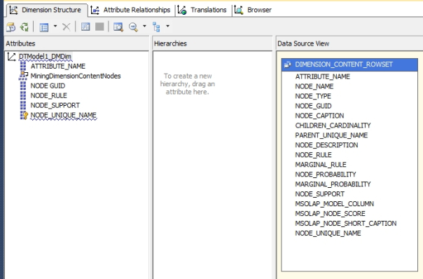

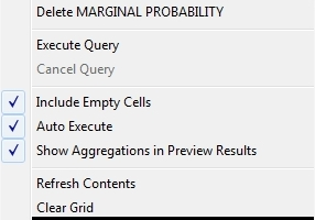
                Even after including these columns, you may not see any worthwhile data depicted in the cube’s Browser tab till you right-click the white space in the table and check the Include Empty Cells command, as depicted in Figure 4.

Figure 4: Include Empty Cells

                Data mining dimensions are of limited use in their current form, however, because of a welter of serious inadequacies. As mentioned before, your data will have to be imported from a cube instead of a relational database, but it can also only be exported to a cube, not into a relational table; even within SSAS, you’re limited to incorporating it is a dimension, not a fact table. Furthermore, they only work with four of SQL Server’s nine data mining algorithms, Decision Trees, Clustering, Sequence Clustering and Association Rules, so we’re crippled right off the bat. One of these is narrowly specialized, as discussed in A Rickety Stairway to SQL Server Data Mining, Algorithm 8: Sequence Clustering, and another is a brute force algorithm that is high popular but appropriate only in a narrow set of use cases, as explained in A Rickety Stairway to SQL Server Data Mining, Algorithm 6: Association Rules. Furthermore, the data provided in mining dimensions comes solely from the common metadata format I introduced in A Rickety Stairway to SQL Server Data Mining, Part 0.1: Data In, Data Out. As I reiterated in each individual article on the nine algorithms, the format is capable of holding apples and oranges simultaneously (like a produce stand), but it comes at the cost of a bird’s nest of nested tables and columns which change their meaning from one algorithm to the next, or even one row to the next depending on the value of such flags as NODE_TYPE and VALUETYPE. The first instinct of anyone who comes from a relational background is to normalize it all, not necessarily for performance reasons, but for logical clarity. If you’re among this crowd, then you’re in luck, because the scripts I’m providing here will allow you to follow those instincts and import all of your mining results into relational tables.

                The concept is really quite simple, at least initially: you create a linked server to your SSAS database using sp_addlinkedserver or the GUI in SQL Server Management Studio (SSMS), then issue DMX queries through OpenQuery. For explicit directions, see the SQLServerDataMining.com webpage Getting Data Mining Results into SQL Tables posted by the user DMTeam on Oct. 24, 2008, but there’s not much left to say about that end of it. The difficult part is formatting your DMX correctly, which can be challenging enough in an SSMS DMX Query window. There are many idiosyncrasies to the language which take getting used to, such as the odd necessity of putting brackets around the PARENT_UNIQUE_NAME column in all situations, the difficulty of scoping FLATTENED columns from NODE_DISTRIBUTION tables and a dozen others. One of the most nagging limitations is the inability of SQL Server to import its own SSDM results using the standard Microsoft OLE DB for Analysis Services data provider, which crashes whenever #IND (indeterminate) or NaN values are encountered in the mined data. The workaround I’ve developed currently requires you to have a copy of Microsoft Excel on your SSAS server because it uses Excel functions to format the #IND and NaN values correctly, but I will probably post a better solution that doesn’t require Excel fairly soon, now that I know how to write SSAS stored procedures. This can be a nightmare to debug, but the scripts I’ll provide take care of the problem for you. Debugging DMX in its native environment is difficult enough, but trying to track down a single error in a query that’s twenty lines long can be a mind-numbing experience when it’s nested inside a T-SQL OpenQuery statement. For all intents and purposes, you’re then also dealing with tracking endless quote marks just as you would with dynamic SQL. If you want to persist the results you’re going to have to use either sp_executesql or INSERT EXEC to get them into a temporary table, thereby adding another layer of quote marks to keep track of.

                The scripts I’m providing here relieve you of most of this burden of coding your own DMX, with the exception of prediction queries. These are handled by the PredictionQuerySP stored procedure I’ve also incorporated, which allows you to execute your own DMX queries in T-SQL, including those with functions that require quote marks, by doubling them like so: EXEC Mining.PredictionQuerySP‘MonitoringLS’, ‘SELECT ClusterProbability(”Cluster 1”) FROM [ClusteredDenormalizedView1Model2]‘. This code can be downloaded here, along with the other stored procedures for importing DMX data into T-SQL. The code was designed with SSMS T-SQL queries in mind, but it can be easily updated to accommodate queries submitted from other data access tools that don’t require double quoting, by adding a simple bit flag and IF statement. Aside from prediction queries, you need not write your own DMX at all, since the eight ImportContent stored procedures (two of the nine algorithms, Logistic Regression and neural nets, share the same procedure and table structure) I’m providing here encapsulate the whole process of transferring your mining results directly into the relational tables created by the companion Data Definition Language (DDL) scripts. There are also procedures and corresponding tables to import any information DMX queries can provide about mining structures, models, their columns and parameters. The procedures also take care of the messy work of normalizing all of SSDM’s nested tables into hierarchies of relational tables. I came up with this solution just a few weeks ago, after I tried to resuscitate a bunch of ad hoc scripts I’d written over the years for this article, only to realize that a more comprehensive and integrated architecture would make more sense. That left me no time to incorporate the necessary error checking or transactions in the procedures, add appropriate nonclustered indexes on the tables, try performance tuning, or any other such considerations. Don’t depend on these scripts until you’ve verified the accuracy of their results first. There are guaranteed to be mistakes in the code, which is a hodgepodge of dynamic SQL, CTEs, MERGE statements and multiple instances of a workaround I developed for the silly limitations Microsoft put on nested INSERT EXEC statements. Feel free to update it to your liking; just please give me credit when possible, because I’d like to get paid at some point for investing all of this energy learning yet another field. I intend to upgrade the scripts on my own for the purely selfish reason that they will help save me the time of writing any more DMX, except in the case of prediction queries. If there’s sufficient interest, I’ll post my revisions here. There’s no reason why we have to reinvent the wheel with each DMX query, when we can write all we need in one big guzzle like this, then store it in a single standardized, interchangeable format. The DDL statements to create the schema in Figure 5 are available here.

Figure 5: Schema v. 0.1 for Importing DMX into Relational Tables (click to enlarge)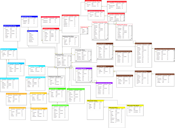

                Your first task in importing SSDM results into this relational schema is to start at the top of the object model and create a new row for your SSAS database in the Mining.SSASDatabase; I haven’t created a stored procedure for this yet, because the metadata for this table is not yet set, so its really only useful at this point for generating identity foreign keys for the MiningStructureTable column SSASDatabaseID. Then use Mining.ImportStructureTableSP to create or update your list of mining structures, by supplying the procedure with the linked server and SSAS database names. At present I haven’t added code to simplify the process any further, so you’ll have to use the identity value generated for a particular structure when running Mining.ImportColumnTableSP and Mining.ImportModelTableSP, which gets the column information and collection of mining models in a single structure. The latter procedure also records the algorithm settings for a particular model, but the model column information will have to be retrieved by supplying the model identity value auto-generated by Mining.ImportModelTableSP to Mining.Import.ModelColumnTableSP. Once these steps are complete, you can import all of your model’s processing results into the appropriate table type, by choosing from one of the following stored procedures based on the model’s selected algorithm: ImportAssociationRulesModelContentSP, ImportClusterModelContentSP, ImportDecisionTreesModelContentSP, ImportLinearRegressionModelContentSP, ImportNaiveBayesModelContentSP, ImportNNModelContentSP and ImportTimeSeriesModelContentSP. They all take an identical set of parameters, including the linked server name, database name and model identity value, like so: EXEC [Mining].[ImportLinearRegressionModelContentSP]‘MonitoringLS‘, ‘MonitorMiningProject’, 18.

                What you can you do with the data once it’s been imported into relational tables? The sky’s the limit. You could create customized views of the results and apply fine-grained security access rights to them; perform sophisticated ANOVA analyses of your mining results; do custom clustering operations; slice and dice the data with the exciting new T-SQL windowing functions; or even build views to compare the intercepts of your regressions across models, or models applying different algorithms, should that prove meaningful to you. Best of all, you can then feed the data into the fact tables and dimensions of an SSAS cube – including the NODE_DISTRIBUTION table data, which you can’t extract through ordinary data mining dimensions – then mine the results again. You could conceivably continue this process recursively, if you had the need and the computational resources. As I explained in A Rickety Stairway to SQL Server Data Mining, Part 0.1: Data In, Data Out, data mining algorithms consist of combinations of statistical building blocks, which could conceivably be arranged in an infinite array of permutations. This whole series is predicated on the idea that a person without a doctorate in statistics can still use these algorithms and their building blocks without understanding their inner workings, as long as they grasp their uses – just as a driver only needs to know what a brake and steering wheel do, not how to reverse engineer them. Therefore I can’t predict what combinations of statistical building blocks you may find useful for a particular project, only that incorporating the results into relational tables will give you much greater freedom to apply them as you see fit.

              SSDM is impressive, but you reach the limits of what you can do with the data once you include it in a data mining dimension or depict it in the GUI; by importing the data into other tools, you can not only present the results differently, but perform further analysis. In my next post, we’ll make mention of four DMX stored procedures we have yet to cover, since they’re advanced means of performing validation tasks on mining models. After that we’ll get into ADO.Net, SSIS tasks, XMLA, Reporting Services and other such alternative means of accessing and extending SSDM programmatically. Functionally, writing custom code and model validation ought to come after learning how to use the nine algorithms correctly, since we can’t validate or retrieve what hasn’t yet been processed. Writing DMX and accessing SSDM with tools like SSIS is not an absolute necessity though, because users can always depend on the GUI tools to view their mining results, as explained in previous posts. It is less practical to do without model validation though, since this is a critical step in the mining process. Why should we rely on the results of faulty models and waste further server resources on them, when statistical and programmatic means are already available to us that can tell us if they’re defective? Stay tuned for that essential step up this long stairway. After that point we will be up the ladder to the roof and practically doing cartwheels on the chimney, which will be the ideal point for a final tutorial or two to close out the series, on the arcane topics of Predictive Model Markup Language (PMML) and plug-in algorithms.