In this Level we will continue the introduction to the MDX time / date series functions group we began in Level 11: MDX Time/Date Series Functions: PeriodsToDate() and Derivative Shortcut Functions. As we discussed there, many business requirements revolve around the performance of analysis within the context of time / date. And while we have seen simple approaches to meeting examples of these requirements (such as determining values for a prior, current, last, etc., reporting period) by using the .CurrentMember, .PrevMember and .NextMember and other functions, this works mainly because the time / date dimension provides a natural (and intuitive) platform for the demonstration of many functions such as these.

Because the need to analyze and report upon data within the context of time / date is pervasive, MDX provides a specialized group of time / date series functions to meet these needs. In Level 11, we gained exposure to the syntax and operation of the PeriodsToDate() function, and then discussed the specialized, predefined “shortcut” functions that are based upon it, including YTD(), QTD(), MTD(), and WTD(). In this Level, we will continue our hands-on exposure to the MDX time / date series functions group with the introduction of the OpeningPeriod() and ClosingPeriod() functions.

We discussed, in our last Level, that we become acquainted early on with the need to perform virtually any data analysis we undertake with reference to time. Examples abound, including the analysis of growth (for instance in revenues or expenses) over periods in time (say, between the years 2007 and 2008). Other common examples within accounting and finance circles include requirements to present year-to-date totals, averages or other accumulations. The common factor in these analytical needs is time, and the primary mission of the time functions is to navigate within the time / date dimension.

The time series functions are specifically designed to support time- and / or date-based analysis. (They are largely applied to dimensions of the “Time” type, but, as we noted in Level 11, can be applied to other dimensions as well – particularly those functions that, unlike the “shortcut” functions like YTD(), QTD(), etc., do not have built-in argument assumptions.) The idea is, again, to allow us to navigate within the time / date dimension to such places as “this month last year,” “the first month in the quarter,” or “our current point in this year, last year.”

For many accounts (such as Fixed Assets, Inventory, and Purchases), and for various other quantities besides dollar amounts that we might maintain (such as headcount, quantity, and so forth) in our systems, balances are maintained up to the current point in time / held at various points in time. A common example is an end of the month balance for a department's employee population, or a total quantity on hand (as of a given date) for a part, say that we stock in a Repair Parts account for use in maintaining our manufacturing equipment. Another common instance might be a value to support our monitoring of the balance in inventory of a good that we intend to sell, to ascertain potentially declining turnover, which might indicate declining market share and obsolescence concerns.

These measures are often analyzed in terms of opening and closing balances for various reasons, particularly at the close of a financial year, but under other time parameters as well. MDX provides an excellent means for referring to the opening and closing points in any given time range / interval that lies within the dimensional structure of our cubes. The OpeningPeriod() function affords us a ready means to navigate to the first member of the day level (as an example) from our position at any time member / level coordinate. The ClosingPeriod() function provides similar access to (as an illustration) the last month-level member – and the balance assigned to that member – within a given year. Moreover, and often useful when working with other MDX time series functions, is that the output of the OpeningPeriod() and ClosingPeriod() functions can serve, respectively, as beginning and end point members, within the time / date dimension, that represent ends of a specified range, across which we can easily aggregate values and so forth.

In this Level we'll become acquainted with the OpeningPeriod() and ClosingPeriod() functions, continuing to address, where useful, some of the common considerations of time / date functions as a part of our exploration. In getting familiar with OpeningPeriod() and ClosingPeriod(), we'll examine the syntax structure with which we employ each, together with illustrative examples of each in practice exercises. At the conclusion of each exercise we perform within the practice session, we'll discuss the MDX results we obtain.

The OpeningPeriod() Function

The OpeningPeriod() function, according to the Microsoft Developer Network, “returns the first sibling among the descendants of a specified level, optionally at a specified member.” OpeningPeriod(), like other functions I include in referring to the “Time / Date series” group, is primarily intended to be used with the time / date dimension, but can actually be used with any dimension.

If a Level Expression is supplied, OpeningPeriod() uses the hierarchy containing the specified level and returns the first sibling among the descendants of the specified level's default member. When we supply both of the function's two arguments, Level Expression and Member Expression, OpeningPeriod() returns the first sibling among the specified member's descendants that exist at the specified level within the hierarchy that contains it. If neither Level nor Member Expression is supplied to OpeningPeriod(), the function looks to the single dimension in the model with a Type of Time, and assumes the default level of that dimension for purposes of operation.

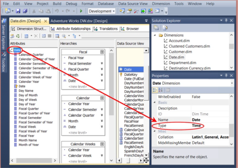
Illustration 1: Dimension Type Property Set to “Time” for the Date Dimension, as Found in the Adventure Works Sample Cube (Partially Expanded)

Putting OpeningPeriod() to work is not difficult, once we grasp its general syntax and operation. And like PeriodsToDate() (which we explored in Level 11: MDX Time/Date Series Functions: PeriodsToDate() and Derivative Shortcut Functions ), OpeningPeriod() enables us to meet very common business needs where the concept of time / date is involved. An obvious example is the calculation of a “beginning balance:” The calculation of this value would likely require the return of the first sibling (or “opening period”) at the Calendar Quarter level of the Calendar hierarchy of the Date dimension.

We might accomplish the same result through other, less direct ways, of course, but OpeningPeriod() is obviously intuitively named, and specifically designed, for what is a common requirement in the business environment. For that matter, a similar, somewhat “opposite direction” function for OpeningPeriod(), the ClosingPeriod() function, exists in MDX to meet an equally common business need: to return the “closing” (or last sibling) as opposed to the “opening” (first sibling) that we see at work in OpeningPeriod().

Syntactically, two arguments are placed within the parentheses to the right of OpeningPeriod, as shown here:

  OpeningPeriod( [ Level_Expression [ , Member_Expression ] ] )

The function returns the first sibling of the descendants of the Member_Expression belonging to the Level_Expression. The following example expression would return the first month of year 2008:

OPENINGPERIOD(
   [Date].[Calendar].[Month], 
      [Date].[Calendar].[Calendar Year].[CY 2008]
          )

Let's extend the above function into a working example. With this example, focus on understanding the syntax, and the dataset that it returns, simply by performing a review. We'll get hands-on practice with the function in the examples that follow this one.

/*  SMDX012-000-Example:  Employ OpeningPeriod() function to return the opening period balance for a specified (in slicer) measure, Reseller Sales, at the Calendar Month level for Calendar Year member 2007    */SELECT 
   OPENINGPERIOD ([Date].[Calendar].[Month], 
      [Date].[Calendar].[Calendar Year].[CY 2007]) ON 0
FROM
   [Adventure Works]  
WHERE
   ([Measures].[Reseller Sales Amount])

The dataset returned would appear as depicted:

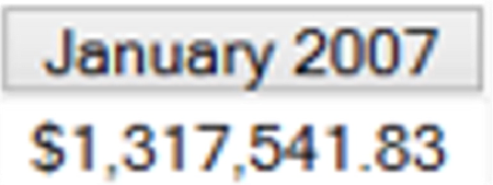
Illustration 2: Example Result Dataset Using the OpeningPeriod() Function

To summarize the action above briefly: The OpeningPeriod() function is used in this case to return, on the column axis, the first sibling of the descendants of the Member_Expression, [Date].[Calendar].[Calendar Year].[CY 2007], belonging to the Level_Expression, [Date].[Calendar].[Month]. The value of the specified measure (per the Where clause), Reseller Sales Amount, for January 2007 (the first month of calendar year 2007) is therefore returned.

Let's begin our hands-on exposure to OpeningPeriod(), to reinforce our understanding of the basics we've discussed. We will, as is typical within this series, work with the MDX Query Editor in SSMS, as our tool for constructing and executing the MDX we examine, and for viewing the result datasets we obtain. If you are not sure how to set up SSMS in Analysis Services, see Stairway to MDX - Level 1: Getting Started with MDX, where we detail the steps in a manner that will be largely identical for SSAS 2008R2 and above.

We'll kick off our practice session with an exercise that employs OpeningPeriod() in a rudimentary way, to demonstrate its basic operation: Let's say that a business analyst with our hypothetical client, Adventure Works Cycles, who is learning how to craft MDX queries in pursuit of meeting day-to-day analysis and reporting requirements, has asked that we assemble a query to demonstrate the “default” action of the OpeningPeriod() function in a case where we do not supply a second argument ( a Member Expression) within the function. We will accommodate him with our first practice exercise.

1. Click / select the Adventure Works cube in the SQL Server Management Studio (“SSMS”) Object Explorer.
2. Click the New Query button above the Object Explorer.
3. Type (or copy and paste) the following query onto the new canvas of the Query pane that opens:

/*  SMDX012-001:  Use OpeningPeriod() function without Member_Expression to 
      demonstrate default behavior in the return of Reseller Sales Amount */SELECT 
   {OPENINGPERIOD ([Date].[Calendar].[Month])} ON 0
FROM
   [Adventure Works]  
WHERE
   ([Measures].[Reseller Sales Amount])

Our input appears in the Query pane.

Illustration 3: Initial Practice Query, Employing OpeningPeriod(), in the Query Pane

4. Click the Execute (!) button in the toolbar.

The Results pane is populated by Analysis Services, and the dataset appears, as partially shown.

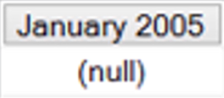
Illustration 4: Example Result Dataset Using the OpeningPeriod() Function

The query has returned the measure specified in the Where clause for the opening period at the Calendar Month level for the Calendar hierarchy (which contains the specified level expression of [Date].[Calendar].[Month] ) of the Date dimension. Because no Member Expression is specified, OpeningPeriod() has simply used the hierarchy (Date.Calendar) containing the specified level, [Date].[Calendar].[Month], and returned the first sibling among the descendants of the [Date].[Calendar].[Month] default member, which is January of the earliest year in the cube (2005).

As an aside, if we juxtapose the month members with the Reseller Sales Amount in an independent query, we can easily verify that the value we see returned (null) is correct: It appears that Adventure Works had no Reseller Sales activity in their first year of operation until the month of July – as it turns out, the beginning of the corporate fiscal year.

Illustration 5: Verification of the January 2005 Balance

5. Save the query by selecting File Save MDXQuery1.mdx As …, naming the file SMDX012-001.mdx, and placing it in a meaningful location.

At this point, let's get some more hands-on exposure with OpeningPeriod(), this time in a more extended application of what we have learned. Let's say that the same Adventure Works client colleague approaches us to simply expand upon his first request: he wants to create a query where, instead of leaving the second argument blank (and thus leaving the Member Expression at its default), we provide the second argument, to give him an idea of the possibilities that using the second argument can offer. Let's assemble a query to meet his request.

6. From our current position within the Query Editor, select File New from the top menu.
7. Select Query with Current Connection from the cascading menu that appears next, as shown.

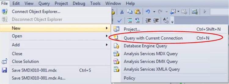
Illustration 6: Creating a New Query via the Current Connection

8. Type (or copy and paste) the following query into the Query pane:

/* SMDX012-002 Create Calculated Measure to determine “Beginning Order Count” using OpeningPeriod() */WITH
MEMBER
   [Measures].[BegOrder Count]
AS
   (
      OPENINGPERIOD(
          [Date].[Calendar].[Date],
  [Date].[Calendar].CURRENTMEMBER
  ),
     [Measures].[Order Count]
  )
SELECT
   {
      ([Measures].[BegOrder Count]),
  ([Measures].[Order Count])
  } ON 0,
   {[Date].[Calendar].[Month].MEMBERS} ON 1
FROM
   [Adventure Works]

The query appears within the Query pane:

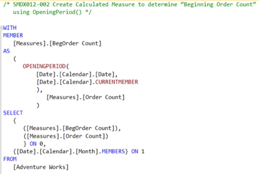
Illustration 7: Query Employing OpeningPeriod() Appears in the Query Pane

9. Click the Execute (!) button in the toolbar, once again.

Analysis Services populates the Results pane, as partially shown:

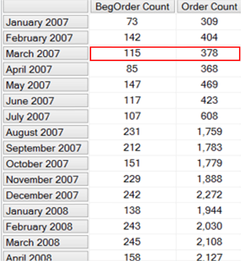
Illustration 8: The Query Results, “Beginning Order Count” Delivered via the Combination of OpeningPeriod() and .CurrentMember (Partial View)

I have highlighted the values for March 2007, as a specific example to reference in the discussion of what's happening. This provides one sample value, for easy confirmation of accuracy / completeness of the returned value of the calculation we have created using the OpeningPeriod() function. Within the calculated member, BegOrder Count, we marshal the combination of the OpeningPeriod() and .CurrentMember functions. The latter, of course, is to specify the current member of the Calendar hierarchy, Date level of the Date dimension.

We bring in the Order Count base measure as well, as a point of comparison to the beginning order count (that is, the count that occurs in the first day of the month under consideration). Side-by-side we can discern the value on the first day of the period as well as count of all orders for the period. We define the row axis with {[Date].[Calendar].[Month].MEMBERS to limit the display returned to “months only.”

10. Save the query by selecting File Save MDXQuery2.mdx As…, naming the file SMDX012-002.mdx, and placing it, as we did with the query we constructed earlier, in a meaningful location.

Let's focus on the March 2007 value and quickly ascertain that we can rely upon the values appearing there. One way is to execute a quick “detail query” that simply lists the values of the base measure under examination, Order Count, by each of the days of March 2007.

SELECT
   {[Measures].[Order Count]} ON 0,
   {[Date].[Calendar].[Month].[March 2007].CHILDREN} ON 1
FROM
   [Adventure Works]

We can easily see from the dataset returned that the Beginning Order Count value for March 2007 that appears in our initial dataset agrees to the Order Count of March 1 in the detailed dataset (115). Moreover, summing the Order Count over all the days of March 2007 give us the total displayed in our month summary dataset above (378).

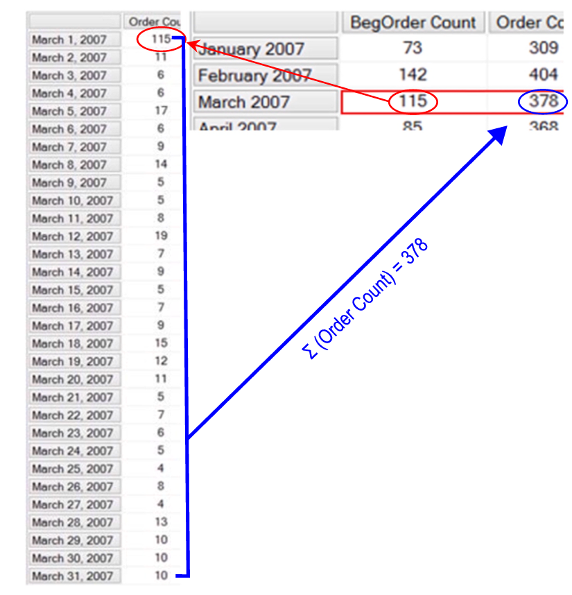
Illustration 9: Verification Query Results: BegOrder Count and Order Count at Month Level Agree to Date Level

Now that we've seen how to use the OpeningPeriod() function, let's take a look at the “equal and opposite” OpeningPeriod() function.

The ClosingPeriod() Function

The ClosingPeriod() function, according to the Microsoft Developer Network, “returns the member that is the last sibling among the descendants of a specified member at a specified level.” ClosingPeriod(), like OpeningPeriod(), and many other functions I include in the “Time / Date series” group, is primarily intended to be used with the Time / Date dimension, but can actually be used with any dimension.

ClosingPeriod(), again like OpeningPeriod(), is a straightforward function with which to work, once we grasp its syntax and operation. And like PeriodsToDate() (which we explored in Level 11: MDX Time/Date Series Functions: PeriodsToDate() and Derivative Shortcut Functions), ClosingPeriod() enables us to meet very common business needs where the concept of time / date is involved. An obvious example of such a need is the calculation of an “ending balance.” The calculation of this value might require the return of the last sibling (or “closing period”) at the Calendar Quarter level of the Calendar hierarchy of the Date dimension.

ClosingPeriod() is intuitively named, as is its counterpart OpeningPeriod(). Although we might craft (via skillful use of its more flexible arguments) the PeriodsToDate() function, or even accomplish its goals through other, less direct ways, ClosingPeriod() is specifically designed for what is a common business requirement.

Syntactically, two arguments are placed within the parentheses to the right of ClosingPeriod, as shown here:

  ClosingPeriod( [ Level_Expression [ , Member_Expression ] ] )

The function returns the last sibling of the descendants of the Member_Expression belonging to the Level_Expression. The following example expression would return the last month of year 2008:

CLOSINGPERIOD(
   [Date].[Calendar].[Month], 
      [Date].[Calendar].[Calendar Year].[CY 2008]
          )

For starters, let's extend the above function into a working example. We'll do some practice exercises next, but, for the time being, examine the function at work in a review of the query below.

/*  SMDX012-001-Example:  Employ ClosingPeriod() function to return the closing period balance for a specified (in slicer) measure, Reseller Sales, at the Calendar Month level for Calendar Year member 2007    */SELECT 
   CLOSINGPERIOD ([Date].[Calendar].[Month], 
      [Date].[Calendar].[Calendar Year].[CY 2007]) ON 0
FROM
   [Adventure Works]  
WHERE
   ([Measures].[Reseller Sales Amount])

The dataset returned would appear as depicted:

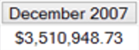
Illustration 10: Example Result Dataset Using the ClosingPeriod() Function

Let's examine what is taking place: The ClosingPeriod() function is used in this case to return, on the column axis, the last sibling of the descendants of the Member_Expression, [Date].[Calendar].[Calendar Year].[CY 2007], belonging to the Level_Expression, [Date].[Calendar].[Month]. The value of the specified measure (per the Where clause), Reseller Sales Amount, for December 2007 (the last month of calendar year 2007) is therefore returned.

To reinforce our understanding of the basics we've discussed, let's begin our hands-on exposure to ClosingPeriod(). We'll resume where we left off earlier with the MDX Query Editor to construct and execute the MDX we examine, and to review the result datasets we obtain. We'll kick off our second practice session with an exercise that employs ClosingPeriod() in a rudimentary way to get a feel for the basics: To simulate a simple business need, let's say our Adventure Works Cycles colleague has asked that we assemble a query to demonstrate the “default” action of the ClosingPeriod() function in a case where we do not supply a second argument (a Member Expression) within the function. This exercise will mirror the first practice exercise we performed with the OpeningPeriod() function in the first half of this level.

1. Click / select the Adventure Works cube in the SQL Server Management Studio (“SSMS”) Object Explorer.
2. Click the New Query button above the Object Explorer.
3. Type (or copy and paste) the following query onto the new canvas of the Query pane that opens:

/*  SMDX012-003:  Use ClosingPeriod() function without Member_Expression to 
      demonstrate default behavior in the return of Reseller Sales Amount */SELECT 
   {CLOSINGPERIOD ([Date].[Calendar].[Month])} ON 0
FROM
   [Adventure Works]  
WHERE
   ([Measures].[Reseller Sales Amount])

Our input appears in the Query pane.

Illustration 11: Employing ClosingPeriod() without Member Expression

4. Click the Execute (!) button in the toolbar.

The Results pane is populated by Analysis Services, and the dataset appears.

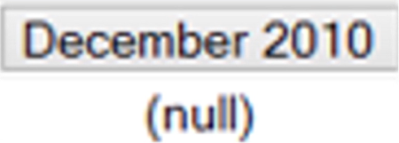
Illustration 12: Result Dataset Using the ClosingPeriod() Function without Second Argument

The query has returned the specified (in the Where clause) measure for the closing period at the Calendar Month level for the Calendar hierarchy (which contains the specified level expression of [Date].[Calendar].[Month] ) of the Date dimension. Because no Member Expression is specified, ClosingPeriod() has simply used the hierarchy (Date.Calendar) containing the specified level, [Date].[Calendar].[Month], and returned the last sibling among the descendants of the [Date].[Calendar].[Month] default member, which is January of the earliest year in the cube (2005).

5. Save the query by selecting File Save MDXQuery3.mdx As …, naming the file SMDX012-003.mdx, and placing it in a meaningful location.

At this point, let's get some more hands-on exposure with ClosingPeriod(), this time in a more extended application of what we have learned. Let's say that the Adventure Works client colleague approaches us again, once more to expand his first request: he wants to create a query where, instead of leaving the second argument of ClosingPeriod() blank (and thus leaving the Member Expression at its default), we provide the second argument, to give him an idea of the possibilities that using the second argument can offer. Let's assemble a query to meet his request.

6. From our current position within the Query Editor, select File New from the top menu.
7. Select Query with Current Connection from the cascading menu that appears next, once again.
8. Type (or copy and paste) the following query into the Query pane:

/* SMDX012-004 Create Calculated Measure to determine “Last Order Count” 
   using ClosingPeriod() */WITH
MEMBER
   [Measures].[LastOrder Count]
AS
   (
      CLOSINGPERIOD(
          [Date].[Calendar].[Date],
  [Date].[Calendar].CURRENTMEMBER
  ),
     [Measures].[Order Count]
  )
SELECT
   {
      ([Measures].[LastOrder Count]),
  ([Measures].[Order Count])
  } ON 0,
   {[Date].[Calendar].[Month].MEMBERS} ON 1
FROM
   [Adventure Works]

The query appears within the Query pane:

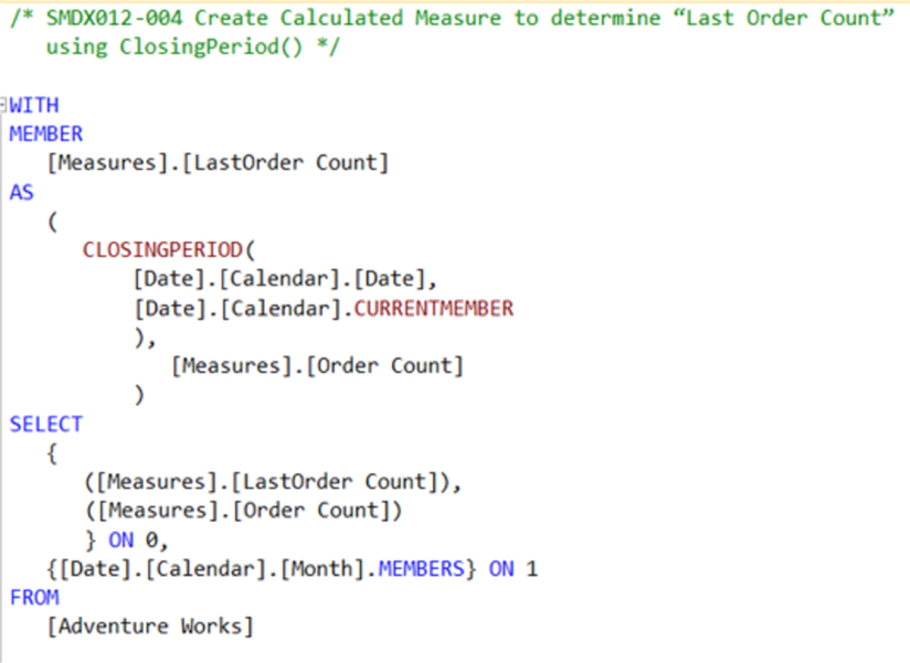
Illustration 13: Query Employing ClosingPeriod() Appears in the Query Pane

9. Click the Execute (!) button in the toolbar, once again.

Analysis Services populates the Results pane, as partially shown:

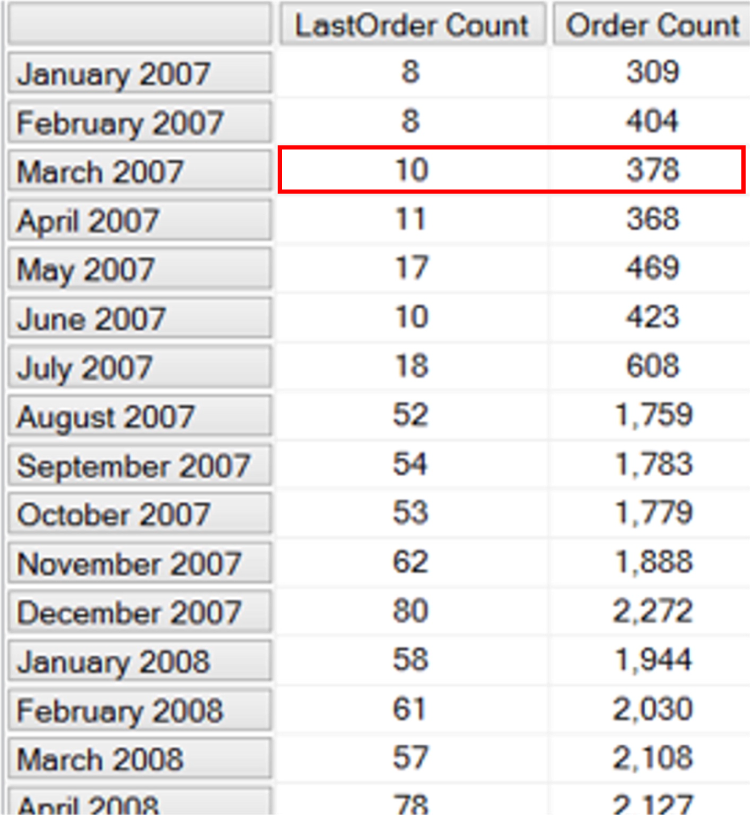
Illustration 14: The Query Results, “Last Order Count” Delivered via the Combination of ClosingPeriod() and .CurrentMember (Partial View)

I have highlighted the values for March 2007, once again, as a particular example to reference in the discussion of what's happening. This will also again provide one sample value, for easy confirmation of accuracy / completeness of the returned value, of the calculation we have created using the ClosingPeriod() function. Within the calculated member, LastOrder Count, we employ the combination of the ClosingPeriod() and .CurrentMember functions as we did for the calculated member in our last practice exercise for ClosingPeriod() earlier. As we used .CurrentMember in that exercise, we use it here: to specify the current member of the Calendar hierarchy, Date level of the Date dimension.

We again bring in the Order Count base measure, here as a point of comparison to the last order count (or the count that occurs in the last day of the month under consideration). Side-by-side we can discern the value on the last day of the period as well as count of all orders for the period. We define the row axis with {[Date].[Calendar].[Month].Members to limit the display returned to “months only.”

10. Save the query by selecting File Save MDXQuery4.mdx As …, naming the file SMDX012-004.mdx, and placing it, as we did with the query we constructed earlier, in a meaningful location.

Let's focus, once again, upon the March 2007 value and gain comfort that we can rely upon the values appearing there. We'll approach this, as before, with a “detail query” that simply lists the values of the base measure under examination, Order Count, by each of the days of March 2007.

SELECT
   {[Measures].[Order Count]} ON 0,
   {[Date].[Calendar].[Month].[March 2007].CHILDREN} ON 1
FROM
   [Adventure Works]

We can easily see from the dataset returned that the LastOrder Count value for March 2007 that appears in the dataset displayed immediately above corresponds with the Order Count of March 31 in the detailed dataset (10). Moreover, summing the Order Count over all the days of March 2007 give us the total displayed in our month summary dataset above (378).

11. Exit SSMS as desired.

The OpeningPeriod() and ClosingPeriod() functions remain a pair of useful, albeit somewhat specialized, time series functions. Since the release of SSAS 2008, other functions achieving their intended ends are often chosen: FirstChild() or FirstNonEmpty() for OpeningPeriod(), and LastChild() or LastNonEmpty() for ClosingPeriod(). While OpeningPeriod() and ClosingPeriod() continue to remain fully functional, these new aggregate functions tend to be selected often, due to added features, to identify the starting and ending periods so critical to much financial analysis. Whatever your leanings in this regard, understanding the concepts behind the functions is vital to the maintenance of a flexible, robust MDX skillset.

Summary

In this Level, we continued an introduction to the time / date series functions group that we began in Stairway to MDX Level 11: MDX Time/Date Series Functions: OpeningPeriod() and Derivative Shortcut Functions. In continuing our exploration of some of the common considerations of time / date functions, together with the options that MDX offers us as support in meeting related business needs, we introduced the OpeningPeriod() and ClosingPeriod() functions as a means for referring to the opening and closing points, respectively, in any given time range / interval that lies within the dimensional structure of our cubes.

In getting familiar with OpeningPeriod() and ClosingPeriod(), we examined the syntax structure with which we employ each, as well as other details of its operation. We gained the know-how needed to take advantage of the OpeningPeriod() and ClosingPeriod() functions through the typical Stairway to MDX practice exercises, whereby we constructed queries that used each, and then examined the results datasets those queries delivered. Throughout the Level, we continued to lay the foundation for our ongoing examination of time / date series functions and expressions, together with other capabilities of MDX to help us to meet typical business needs.