In this Level, we expose the DAX DISTINCT() function, which, like the FILTER() function we examined in Level 2: The DAX COUNTROWS() and FILTER() Functions and More About Calculated Columns and Measures, returns a single-column table of results, and therefore most commonly serves as an argument to other (typically aggregation-rendering) functions. When applied to a column, DISTINCT() returns a table containing the unique values contained within the targeted column. This means, of course, that DISTINCT() removes any duplicates before returning the subset table of distinct values.
We’ll discuss ways in which DISTINCT() can be employed, first in a “standalone” example for the function, and then in situations where we it with other functions, to achieve a result similar to something we might need to generate for clients or employers in our own environments. As part of our exploration of the DISTINCT() function, we will:
- Examine the syntax surrounding the function;
- Undertake illustrative examples of the uses of the function in practice exercises;
- Briefly discuss the results datasets we obtain in the practice examples.
In addition to introducing this new DAX function, we will examine the output we obtain via a calculated column we construct within the Power Pivot window in the practice session that follows. We will further create a calculated measure, within a new PivotTable, that uses the DISTINCT() function (in combination with another DAX function) to replicate the behavior that we have examined in the calculated columns created in the PowerPivot window. As is typically true within the Levels of this series, we will compare and contrast calculated columns and calculated members in general, and discuss criteria to consider in choosing which of these calculation types to use to meet requirements we encounter in supporting employers and clients.
Preparation for the Levels of the Stairway to PowerPivot and DAX Series
As we’ll note throughout, to obtain the most benefit from the Levels of the Stairway to PowerPivot and DAX series, you will need to have installed the PowerPivot for Excel 2010 add-on on your machine. You will also need to have installed SQL Server 2008 or above (including Analysis Services) and the respective relational and Analysis Services samples on your local machine, or have the client portions of each on your machine with access to the rest on a server. To perform all Levels of preparation, see the installation section of the charter Level of this series, Level 1: Getting Started with PowerPivot and DAX.
Preparation for the Practice Exercises in this Level
Once we’ve got the PowerPivot for Excel 2010 add-in, SQL Server 2008R2 and the samples noted above installed, we’re ready to perform the practice exercises within this Level. Importing the sample database and taking other preparatory steps are critical to providing the environment required to successfully complete this Level, and should be performed before beginning. Because we will work with different data sources throughout this series, the steps of environment preparation will be repeated in various steps. The objective is to make each Level a freestanding session that can be completed independently of other Levels, so that you can focus upon gaining exposure to the specific skills required to meet your own immediate requirements efficiently. Where appropriate, references to functions, procedures and other details will be supplied, but the objective of each Level is to focus upon one or more specific DAX functions and / or PowerPivot / PivotTable procedures to satisfy needs that mirror requirements you encounter in our own business environments.
Let’s open PowerPivot and import our data by taking the steps below. This will put us in position to begin learning the material in this Level.
1. From the Start menu, select Microsoft Excel 2010.
2. Above the Excel ribbon, click the PowerPivot tab, as shown.
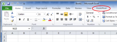
Illustration 1: Click the PowerPivot Tab …
The PowerPivot ribbon appears.
3. Click the PowerPivot Window Launch button, appearing at the left of the newly appearing PowerPivot toolbar, as shown.

Illustration 2: The PowerPivot Window Launch Button on the PowerPivot Ribbon …
The PowerPivot window, containing its own ribbon, opens atop the existing Excel spreadsheet, assuming the name of the workbook as its own name, as depicted below.
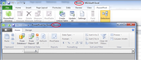
Illustration 3: The PowerPivot Window, Associated with the Workbook, Appears
As we noted in Level 1: Getting Started with PowerPivot and DAX, it is in the PowerPivot window that we load and prepare the data with which we will be working (or will continue working, if data is already added to the workbook). We will typically build a relational model here (even when we import other-than-relational sources, such as Analysis Services data, text files, .RSS feeds, and so forth). As we also noted in Level 1, the PowerPivot window displays the tables on individual, tabbed sheets, and is the central place where we import tables, create relationships, maintain column data types and formats, and view, as needed, the data that underlies our data model, among other actions.
Next, we’ll designate a source from which to import data.
4. Click the From Database button on the Home tab of the PowerPivot window.
5. Select From SQL Server on the drop-down menu that appears next.
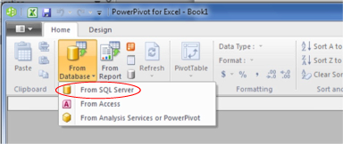
Illustration 4: Select “From SQL Server” in the From Database Dropdown
The Table Import Wizard dialog opens next.
6. In the top input box, titled Friendly connection name, type (or copy and paste) the following:
AdventureWorksDW2008R2
7. Click the selector (downward pointing arrow) on the right side of the box titled Server name.
PowerPivot begins a scan of the machine to detect, and return to the selector, the available server choices.
8. Select the appropriate server for your local environment, or type in the server name / localhost, as appropriate.
9. Enter the authentication as required for the local environment (ideally selecting Use Windows Authentication).
10. Select AdventureWorksDW2008R2 using the dropdown selector to the right of the box titled, Database name, at the bottom of the dialog.
The Table Import Wizard dialog, with our input, appears similar to that depicted below.
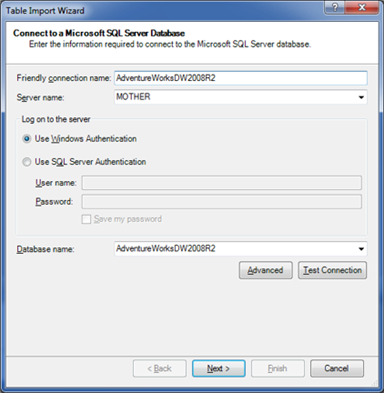
Illustration 5: The Table Import Wizard Dialog, with Our Input
11. Click the Test Connection button underneath the Database name selector.
A message box appears, indicating that the test connection has succeeded.

Illustration 6: “Test Connection Succeeded”
12. Click OK to dismiss the message box.
13. Click the Next button at the bottom of the Table Import Wizard dialog.
14. On the dialog that appears next, labeled Choose How to Import the Data, leave the radio button at its default of Select from a list of tables and views to choose the data to import, as shown.
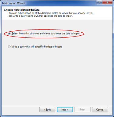
Illustration 7: Choose “Select from a list of tables…” Option for Data Import
15. Click the Next button.
PowerPivot loads the tables and views from the AdventureWorksDW2008R2 database into the Select Tables and Views page of the Table Import Wizard that appears next.
16. Select the following tables, by clicking the checkbox to the immediate left of the respective table listing in the dialog:
- DimCustomer
- DimDate
- DimProduct
- DimProductCategory
- DimProductSubcategory
- DimPromotion
- DimSalesTerritory
- FactInternetSales
The Select Tables and Views dialog appears, as partially shown, with our selection and related tables checked.
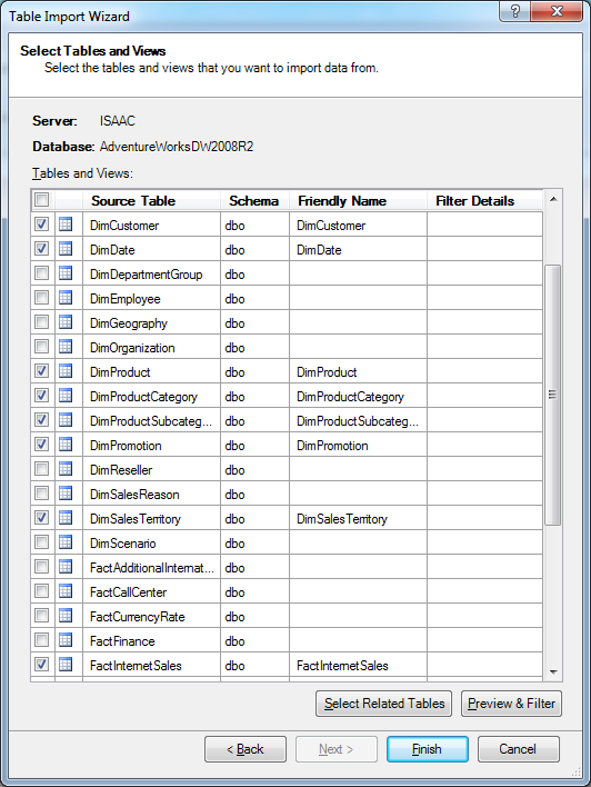
Illustration 8: Selecting Tables (Partial View) …
The idea in these immediate steps is to import enough information into our model to allow us to do some illustrative analysis surrounding the business activities conducted by our hypothetical client, the Adventure Works organization.
17. Click the Finish button.
The import process runs, and then we see a “Success” message, complete with a Details list that indicates population by our choices.
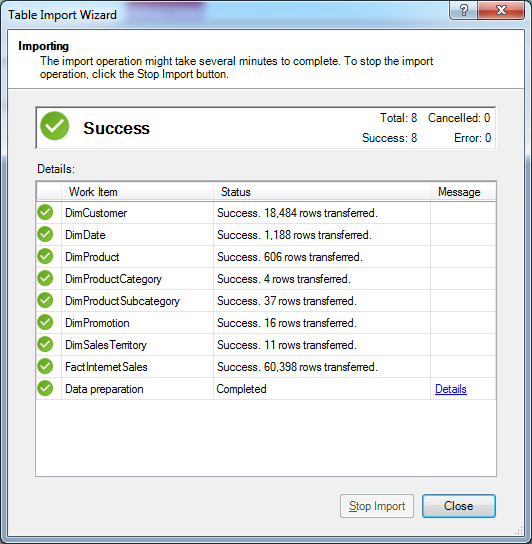
Illustration 9: Success is Indicated, Along with a List of Tables Imported
18. Click Close.
The Table Import Wizard is dismissed, and we arrive at the PowerPivot window once again, where we see the imported data as partially depicted.
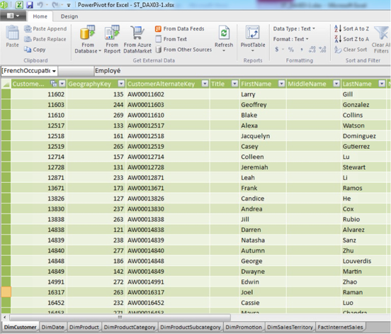
Illustration 10: Imported Data, with a Tab for Each Table
Note that a tab for each imported table has been created in the PowerPivot window (the tabs appear in the bottom left of the window, as seen above). What we are now seeing is not an Excel table, but a view of the efficiently compressed columnar database that PowerPivot uses to store imported tables in memory. For more detailed information about the PowerPivot window itself, please see Level 1: Getting Started with PowerPivot and DAX
19. Click the selector underneath the Quick Access Toolbar (assuming it is in the default, above-the-ribbon position), and to the immediate left of the Home tab in the ribbon.
20. Select Save As from the dropdown menu that appears, as shown in Illustration 11.

Illustration 11: Select Save As from the Selector within the PowerPivot Window …
21. Save the worksheet as ST_DAX03-1.xlsx, placing it in a convenient location.
22. Leave the PowerPivot Window open for the practice session below.
We are ready, at this stage, to get some hands-on exposure to a new DAX functionDISTINCT(), while revisiting functions that we introduced in previous levels, as well as continuing to build experience with the general use of PowerPivot to meet business requirements, in the sections that follow.
The DISTINCT() Function
Introduction
According to the TechNet Library, the DAX DISTINCT() function “returns a one-column table that contains the distinct values from the specified column.” Moreover, according to the same reference, “… duplicate values are removed and only unique values are returned.”
DISTINCT() is a member of the Filter Functions group, whose complex and powerful members enable us to manipulate data context to craft dynamic calculations.
DISTINCT() is highly useful in numerous contexts, and is typically used in conjunction with other functions. An example of a common case, which we’ll see in action later in this Level, is a situation where it provides, in combination with the DAX COUNTROWS() function, a means of generating a distinct count, a feat that was much more difficult to do in Excel prior to the advent of PowerPivot for Excel 2010.
An important consideration when using DISTINCT() – as is the case with many DAX functions – is that the output of DISTINCT() is affected by the current filter context. (We will repeatedly focus upon the concept of context throughout the Stairway to PowerPivot and DAXseries.) For example, if we use the formula in the following example (given the environment we have set up for our practice session) to create a PivotTable measure, the output of the function would change whenever the table was filtered to show only, say, a particular time period or geographical location.
=COUNTROWS(DISTINCT(FactInternetSales[CustomerKey]))
We will explore the syntax for the DISTINCT() function after a brief discussion in the next section. We will then gain some hands-on exposure to its use, within practice examples constructed to support hypothetical business needs. This will allow us to activate what we explore in the Discussion and Syntax sections.
Discussion
To restate our initial explanation of its operation, the DISTINCT() function, when acting upon a specified column, return a one-column table containing the distinct values that are used within that column. Therefore, as part of the function’s operation, duplicate values are removed and only unique values are returned.
DISTINCT() cannot be used to return values into a worksheet column or into a cell. That is, the list of values returned by DISTNCT() cannot be pasted directly into a column. Instead, we pass the results of the function into another function for aggregation, counting, filtering or other desired ends, as we shall see. As we have noted, within the PivotTable, the current filter context affects the results that are delivered by DISTINCT().
Let’s look at some syntax illustrations to further clarify the operation of DISTINCT().
Syntax
Syntactically, in using the DISTINCT() function to return the distinct values contained within a column we specify, the column / column expression upon which we seek to apply the function is specified, within parentheses, to the right of the DISTINCT keyword. The general syntax is shown in the following string:
DISTINCT(<column>)
Putting DISTINCT() to work is intuitive, once we grasp its purpose. When using the function to return the list of distinct values of the column / column expression(“<column>” in the syntax string above) with which it works, we simply enclose the column name or expression in parentheses to the right of the DISTINCT() keyword, as we have noted. We have to keep in mind, of course, that we cannot return the distinct list of members to a column in the simplest sense, but will have to further manipulate the returned list into a single outcome that can be represented in a single column or cell.
For example, let’s get a feel for the general use of DISTINCT() within the DimPromotion tab of the PowerPivot window, where we have performed the imports described in the Preparation section above. Let’s say we want to put DISTINCT() to use in a scenario where we wish to do something conceptual like this:
=DISTINCT(DimPromotion[EnglishPromotionCategory])
When we look at the specified column on the tab, EnglishPromotionCategory, we see the following:
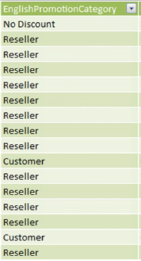
Illustration 12: The EnglishPromotionCategory Column of the DimPromotion Tab
A distinct list of members in this case would consist of the following three Promotion Categories:
- No Discount
- Reseller
- Customer
Knowing what we do about the DISTINCT() function, we realize that, even though this would be the returned list, we cannot expect this three member list to appear in a new calculated column of the tab. For that matter, if we attempt simply to create a column with the syntax =DISTINCT(DimPromotion[EnglishPromotionCategory]), we obtain an error (#ERROR in each of the rows of the proposed calculated column), for the reasons we’ve already discussed.
On the other hand, should we use the function in the intended way, and enclose it within a “wrapper” function which, as a characteristic, returns a single value, we would find that the three member set that we expect to be the conceptual result of the syntax we are considering is, indeed, “held,” and can be operated upon if passed to a function that returns an acceptable output. We will see an example of this in the practice section that follows.
Practice
To reinforce our understanding of the basics we have covered so far, we will use the DISTINCT() function within the definition of a couple of calculations, first via a calculated column within a tab of the PowerPivot window, and then via a calculated measure within a PivotTable of a worksheet within the associated Excel workbook. We will examine its use in combination with a function we introduced in Level 2: The DAX COUNTROWS() and FILTER() Functions and More About Calculated Columns and Measures. The intent, as in all the practice sessions of the Stairway to PowerPivot and DAX series, is to demonstrate the operation of each of the functions we examine in a straightforward, memorable manner.
We will turn to the Excel worksheet we prepared earlier as a platform from which to construct and execute the DAX we examine, and to view the results we obtain.
PowerPivot Calculated Column
1. Return to the worksheet we created in the Preparation for the Practice Exercises in this Level section above, ensuring that the PowerPivot Window is open, where we left it earlier.
2. Click the DimPromotion tab.
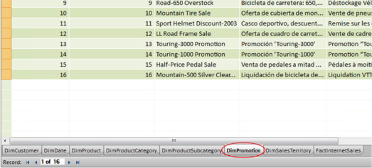
Illustration 13: Click the DimPromotion Tab …
3.Click the top row in the column labeled "Add Column,” which appears on the far right side of the tab, as shown.
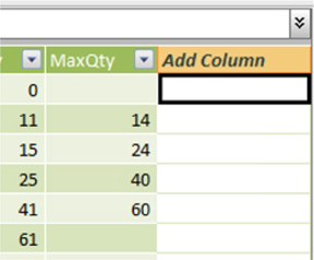
Illustration 14: Click the Top Row in the Column Labeled “Add Column”
4. Select the function button (“fx”) to the left of the formula bar next.
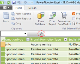
Illustration 15: Select the Function (fx) Button …
The Insert Function dialog appears.
5. Click the downward pointing arrow on the selector appearing atop the dialog under the Select a category label.
The following DAX function categories appear:
All
Date & Time
Math & Trig
Statistical
Text
Logical
Filter
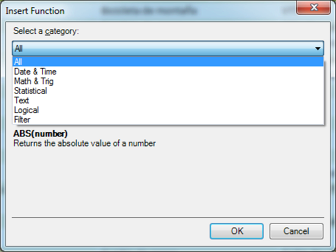
Illustration 16: Insert Function Dialog with Expanded Category Selector
6. Select the Statistical category.
7. In the Select a function list that populates for the Statistical category, select the COUNTROWS() function, as shown in Illustration 17.
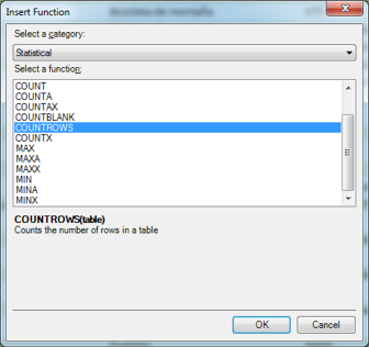
Illustration 17: Select the COUNTROWS() Function
8. Click OK to confirm the selection and dismiss the Insert Function dialog.
The COUNTROWS keyword, proceeded by the “=” operator and followed by a left parenthesis ( “(“ ) appears in the formula bar, with a function usage tooltip appearing just underneath the function.
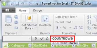
Illustration 18: The Beginning of the COUNTROWS() Function, along with Tooltip, Appears
9. Because we know that we need now to add the appropriate table name / expression, begin to type in “DimPromotion.”
As we begin to type the table name, AutoComplete immediately presents us with a list of functions and tables from which to select, as shown.
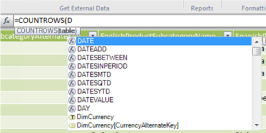
Illustration 19: Functions / Tables as Suggested by AutoComplete …
10. Scroll to DimPromotion, and click to select it, as depicted in Illustration 20.
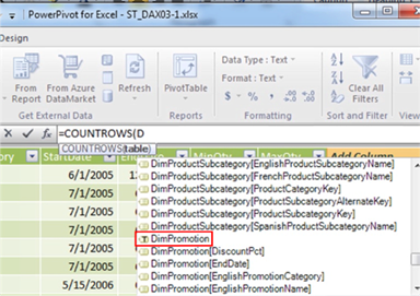
Illustration 20: Select the DimPromotion Table …
We note again that the “T” within the icon preceding the table name identified this as a table, versus a table column, label (the columns are preceded by icons without the “T”).
11. Once the selector is dismissed, and =COUNTROWS(DimPromotion appears in the formula bar, type in a closing right parenthesis ( “)“ ) to complete the formula.
A completed formula appears – this is but a “way station” to the ultimate formula using DISTINCT(), of course.
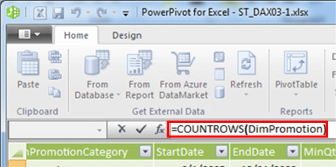
Illustration 21: The Completed Formula Appears
12.Press the Enter key.
The column updates and the formula results appear in each row of the new calculated column (the number 16), as partially shown below.
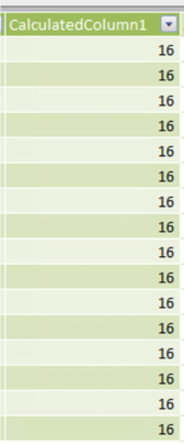
Illustration 22: The Results Appear in Each Row of the New Column (Partial View)
We note that the value “16” makes complete sense, as DimPromotion contains exactly sixteen rows. Let’s name the column in accordance with its ultimate intended purpose, at this juncture.
13. Right-click the new column header label (currently at its default of “CalculatedColumn1”), and select Rename Column from the cascading menu that appears.
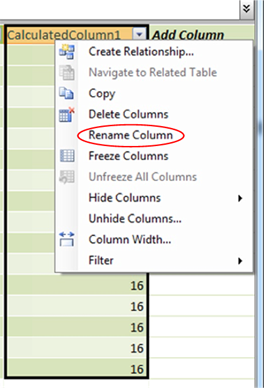
Illustration 23: Renaming the Column to its Ultimate Name
14. Name the newly added column “Dist Ct - Promotions” for “Distinct Count – Promotions.”
Now let’s continue our ultimate objective – to gain hands-on exposure to the use of DISTINCT() to meet a real-world need: the generation of a distinct count. We know that the table contains sixteen rows, and the ROWCOUNT() function has delivered that value, as expected. We wish now, however, to go the next step, and demonstrate how we might obtain a distinct count of the members of a column that does not contain a unique member on each row. Such a column, in this case, is the EnglishPromotionCategory column of the DimPromotion table, which contains only three different categories, No Discount, Reseller, and Customer, as we can readily see upon examination of the column.
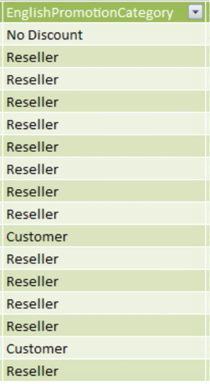
Illustration 24: Three Distinct Category Members
As many of us know, distinct counts have traditionally been difficult in PivotTables. The DAX DISTINCT() function makes this much easier, and it can be employed either here, in the PowerPivot window (in a calculated column), or within the PivotTable (to create a calculated measure). Because the DISTINCT() function, as we have noted, returns a single-column table (in this case, it would have three values in it, No Discount, Reseller, and Customer), we will need to “wrap” the DISTINCT() function within the COUNTROWS() function we have already added, so that the number of rows in the table delivered by DISTINCT() can be counted. Let’s modify the new calculated column to make this happen.
15. At the far right of the same DimPromotion tab, return to the new Dist Ct – Promotions calculated column, clicking the top row in the column to display the formula created in the formula bar.
16. To the right of the left parenthesis (that appears to the right of the COUNTROWS() function) insert the following:
DISTINCT(
17. Remove the right parenthesis that appears in the function bar at the end of the current syntax
AutoComplete displays our selection options at this point.
18.Double-click DimPromotion[EnglishPromotionCategory] from the selection list, as shown in Illustration 25.
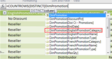
Illustration 25: Modifying the Original Formula …
19. Add two right parentheses (“ )) “) to the right of the formula.
The complete text appears, in the formula bar, at this stage, as shown.

Illustration 26: The Complete Text in the Formula Bar
20. Press the Enter key to generate the contents of the new calculated column.
The new calculated column populates with the number “3,” (the number of unique occurrences in the DimPromotion[EnglishPromotionCategory] column), and appears as shown.
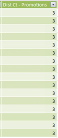
Illustration 27: The Newly Populated “Distinct Count – Promotions”
As most readers of this series are aware by now, a significant strength of PowerPivot environment lies in the fact that the same data and slicers can be shared by multiple PivotTables. Let’s see just how straightforward this is by taking a look, in the section that follows, at a PivotTable example where we can see how to access components with which we have worked so far in this Level of our series. We’ll also look at how to replicate the same logic we employed in the calculated columns we created in this section to create calculated measures in a PivotTable.
PivotTable Measure
As we have noted elsewhere in the Stairway to PowerPivot and DAX series, PowerPivot exists, in its most fundamental and common use, to act as a data source for PivotTables. In this section, we will work further with the DAX functions we have exposed in the PowerPivot calculated column section above, except this time, we will present values and calculations within a PivotTable.
We can begin our work with a PivotTable from either the Excel workbook or from the PowerPivot window. Because we’re already in the latter, we will proceed from there by taking the following steps:
1. From the DimPromotion tab in the PowerPivot window, click the downward pointing arrow on the PivotTable button to cause the drop-down menu to appear, as shown.
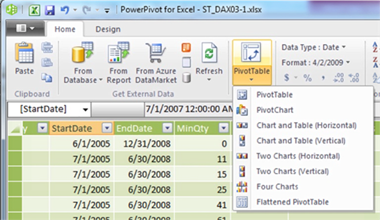
Illustration 28: The PowerPivot Drop-down Menu Appears …
While we will work with examples, at various times throughout our series, of some of the other options we see in the dropdown menu (single PivotChart, Chart & Table, Two Charts, Four Charts, and Flattened PivotTable), we will build a single PivotTable in this session, and most of the practice sessions, of our series, as this will be the most straightforward (and rapid) avenue to getting hands-on exposure to the underlying PowerPivot data and DAX, in general.
2. Click PivotTable in the dropdown menu we’ve exposed (the top selection).
We are returned to the Excel window, where we encounter the Create PivotTable dialog.
3. Ensure that the radio button labeled New Worksheet is selected.
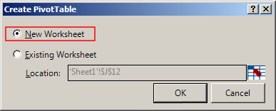
Illustration 29: Ensure the New Worksheet Option is Selected
4. Click OK to accept the setting and dismiss the dialog.
The PivotTable placeholder / canvas, together with the PowerPivot Field List, appear on the new worksheet as depicted (compressed view).
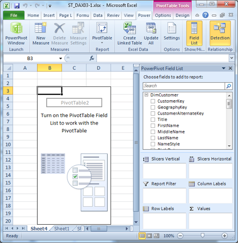
Illustration 30: The PivotTable Canvas Appears on the New Worksheet (Compressed View)
The placement of the new PivotTable is set, by default, to lie within the range of cell B3 to cell D20, which, as we noted in Level 2: The DAX COUNTROWS() and FILTER() Functions and More About Calculated Columns and Measures, occurs for a reason that will become evident many times in the Stairway to PowerPivot and DAX series: to afford space for the insertion of vertical and horizontal slicer button groups to frame the PivotTable, should we make the selections needed to use them. We also see that the PowerPivot Field List, appearing to the right of the PivotTable, contains elements that will be new to those of us that have become familiar with the standard PivotTable Field Lists: two new Slicer zones are now included.
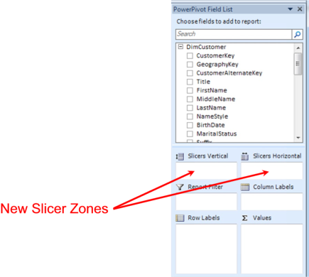
Illustration 31: Two New Slicer Zones Appear in the PowerPivot Field List
NOTE: Because we looked at it for the first time in the last Level of the series, and particularly for those not familiar with standard Excel PivotTables, Table 1 of Level 2: The DAX COUNTROWS() and FILTER() Functions and More About Calculated Columns and Measuresgives a description for each of the areas / zones on the PowerPivot Field List. Other PivotTable basics are discussed there as well.
To gain some exposure to the use of the DAX DISTINCT() function within the PivotTable, we will replicate some of the steps we took with regard to the DimPromotion table, upon which we operated in the PowerPivot window in the earlier part of this Level. In accomplishing this, we’ll see how to approach what we did with the calculated column earlier, but this time we’ll do so with a calculated measure in the PivotTable. Moreover, we will touch upon more PivotTable – specific considerations as we encounter them.
5. Expand the DimPromotion table in the Field List by clicking the “+” sign to its immediate left.
The columns of the table, with which we worked in the PowerPivot window in the section above, appear.
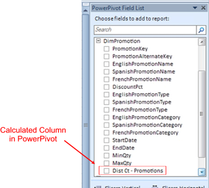
Illustration 32: DimPromotion Table in the PowerPivot Window, Expanded to Show Fields
The last field in the expanded list, of course, represents the calculated column that we created earlier, using a combination of the DAX DISTINCT() and COUNTROWS() functions, in the PowerPivot window. While we could pull this calculation into our new PivotTable like any other field at this point, let’s first examine how to create it as a calculated measure – to demonstrate how to use DAX at the PivotTable level.
6. Within the PowerPivot Field List, right-click the newly expanded DimPromotion label.
7. Select Add New Measure… from the context menu that appears, as shown.
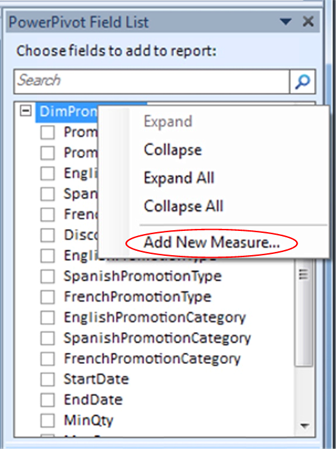
Illustration 33: Select Add New Measure …
The Measure Settings dialog appears.
8. Type (or copy and paste) the following into both the Measure Name and Custom Name boxes of the dialog.
Mx Dist Ct - Promotion
9. Click the function button (“fx”) to the right of the Formula label, above the Formula input box of the dialog.
The Insert Function dialog appears.
10. Click the downward pointing arrow on the selector appearing atop the dialog under the Select a category label.
11.Select the Statistical category within the expanded category selector atop the Insert Function dialog, just as we did in the earlier exercise.
12.Select the COUNTROWS() function, once again, as depicted in Illustration 34.
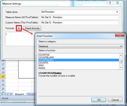
Illustration 34: Select Add New Measure …
13. Click OK to confirm the selection and dismiss the Insert Function dialog.
The COUNTROWS keyword, proceeded by the “=” operator and followed by a left parenthesis, once again, appears in the Formula input box of the Measure Settings dialog.
14. To the right of the left parenthesis (that appears to the right of the COUNTROWS keyword) insert the following:
DISTINCT(
15. Begin to type in DimPromotion … to the right of DISTINCT( .
As we begin to type the table name, AutoComplete again presents us with a list of functions and tables from which to select:
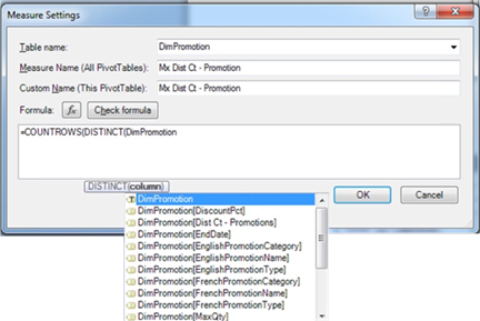
Illustration 35: Functions / Tables as Suggested by AutoComplete …
16.Double-click DimPromotion[EnglishPromotionCategory], as we did at the PowerPivot level earlier, to ensure its selection.
17. Once the selector is dismissed, and =COUNTROWS(DimPromotion[EnglishPromotionCategory] appears in the formula bar, type in two closing right parentheses ( “))“ ) to complete the formula, as we did for the similar calculated column in the PowerPivot window in the earlier section of this Level.
The completed formula string appears, in the formula input box, at this stage, as shown.
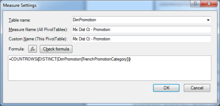
Illustration 36: The Complete Text in the Formula Input Box
18. Click the OK button.
The calculation for the new measure is saved, and the Measure Settings box is dismissed. The new calculated measure, Mx Dist Ct - Promotion, appears in the PowerPivot Field List, underneath the other fields within the expanded DimPromotion fields list. Mx Dist Ct - Promotion (we named it this so as to distinguish it from the calculated column Dist Ct - Promotions that appears above it) comes “preselected:” the check mark is already in the box to the left of the calculated measure (a calculated measure is indicated by the calculator icon to its immediate right), and the new measure appears, by virtue of its selection, in the Values zone (bottom right corner) of the PowerPivot Field List. Finally, because of its being placed in the Values zone, the measure also appears on the spreadsheet, within the PivotTable, where we see the number “3.” The PivotTable environment appears, reflecting these circumstances, as shown.
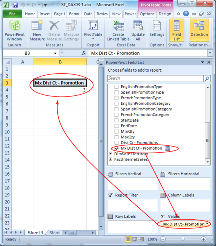
Illustration 37: The PivotTable Environment, Reflecting the Addition of the New Calculated Measure
NOTE: For more information on the mechanics of docking / undocking the PivotTable Field List, as I do in many illustrations to help make them more compact, see Level 2: The DAX COUNTROWS() and FILTER() Functions and More About Calculated Columns and Measures.
Having added a calculated measure to the PowerPivot Field List that is the formulaic equivalent of what we created as our first PowerPivot calculated column in the earlier section of this Level, let’s go a step further and discuss a major difference between the calculated column and the calculated measure we have created – at least when using them within the PivotTable. First, let’s place the two side-by-side for closer examination.
19. Within the PivotTable Field List, click the checkbox to the immediate left of the Dist Ct - Promotions calculation that appears in the list directly above the newly created Mx Dist Ct – Promotion measure.
Checking Dist Ct - Promotions places it in the Values drop zone of the PivotTable Field List, below the newly created Mx Dist Ct – Promotion measure, as well as on the spreadsheet, within the PivotTable, to the right of the Mx Dist Ct – Promotion measure, where it displays the number “48.”
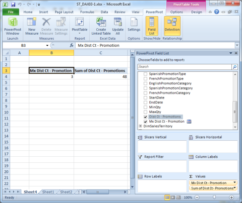
Illustration 38: PivotTable Measure Juxtaposed with Its PowerPivot Calculated Column Counterpart
So why are the values different, when, at their respective levels of computation, they reflect the same formula, and at their respective levels, return the same value? The reason, while relatively straightforward, sometimes causes issues with those new to PowerPivot, and deserves a glance, at this point, as it illustrates a potential stumbling block. It is important to realize that, when we bring a calculation into the PivotTable via the Values drop zone, we need to consider the fact that implicit summing occurs. We note the presence of the summation symbol, ?, an enlarged form of the upright capital Greek letter Sigma, to the immediate left of the Values label atop the drop zone, as well as the default labeling of the selected calculated column as “Sum of [calculation name]”:
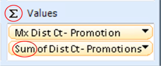
Illustration 39: Default Summing Occurs with PowerPivot Calculated Columns
Noting this, it becomes rather intuitive why we see “48” in the affected PivotTable cell: the sixteen rows of “3” in the PowerPivot DimPromotion tab are being added up to render a total of 48.
We will discuss several related considerations as we explore the concept of context throughout prospective Levels of our series. For now, my point is to illustrate the importance of realizing specifically “what we are asking for” when we leave settings at default, and thereby sum, calculated column selections within the PivotTable environment.
1. From the main menu of the workbook, select File -- Save As …
2. Name the file ST_DAX03-1.xlsx, and save it in a meaningful location.
3. Exit Excel 2010 as desired.
As I emphasize in other Levels, understanding the nature and operation of, the differences between, and the optimal uses for, calculated columns and calculated measures is critical to sound and efficient reporting and analysis when working with PowerPivot. We will work with these concepts throughout the Levels of Stairway to PowerPivot and DAX, embellishing and enhancing our technique as the series evolves. Practice and further experimentation with these and other components will ensure that we become fluent in the many options and opportunities that PowerPivot offers the knowledgeable user.
Summary …
In this Level of the Stairway to PowerPivot and DAX series, we exposed the DAX DISTINCT(), and revisited the DAX COUNTROWS(), functions. We discussed the general purposes and operation of DISTINCT(), and then focused upon using DISTINCT() in general, as well as the illustrating a way to leverage the combination of DISTINCT() and COUNTROWS() to deliver a distinct count – a process that was difficult to accomplish in Excel prior to the advent of PowerPivot and DAX. As part of our discussion, we examined the syntax surrounding DISTINCT(), undertaking a couple of illustrative examples of the uses of the function in practice exercises, and then exploring the results datasets we obtained in the practice examples.
We worked with the combination of DISTINCT() and COUNTROWS() to deliver a distinct count within both a PowerPivot calculated column and a PivotTable calculated measure we built in the section that followed. Once we had replicated, in the PivotTable, the calculated column we had created earlier in the PowerPivot window, we compared and contrasted the value returned by each, explaining the reason behind their difference, and discussing considerations in choosing which of these two calculation approaches to take in meeting business requirements in our own environments.
