The loading of data from a source system to target system has been well documented over the years. My first introduction to an Extract, Transform and Load program was DTS for SQL Server 7.0 in 1998.

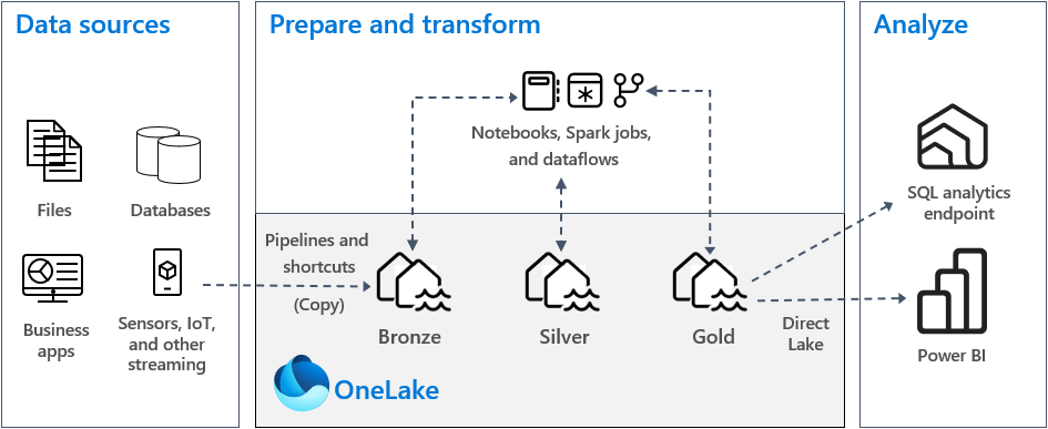
In a data lake, we have a bronze quality zone that is supposed to represent the raw data in a delta file format. This might include versions of the files for auditing. In the silver quality zone, we have a single version of truth. The data is de-duplicated and cleaned up. How can we achieve these goals using the Apache Spark engine in Microsoft Fabric?

Business Problem

Our manager has given us weather data to load into Microsoft Fabric. In the last article, we re-organized the full load sub-directory to have two complete data files (high temperatures and low temperatures) for each day of the sample week. As a result, we have 14 files. The incremental load sub-directory has two files per day for 1,369 days. The high and low temperature files for a given day each have a single reading. There is a total of 2,738 files. How can we create a notebook to erase existing tables if needed, rebuild the full load tables, and rebuild the incremental tables?

Technical Solution

This use case allows data engineers to learn how to transform data using both Spark SQL and Spark DataFrames. The following topics will be explored in this article (thread).

1. passing parameters
2. show existing tables
3. erase tables
4. full load pattern
5. testing full load tables
6. incremental load pattern
7. testing incremental load tables
8. future enhancements

Architectural Overview

I borrowed the image from Emily Riederers blog since I liked it. What is the difference between a full and incremental load?

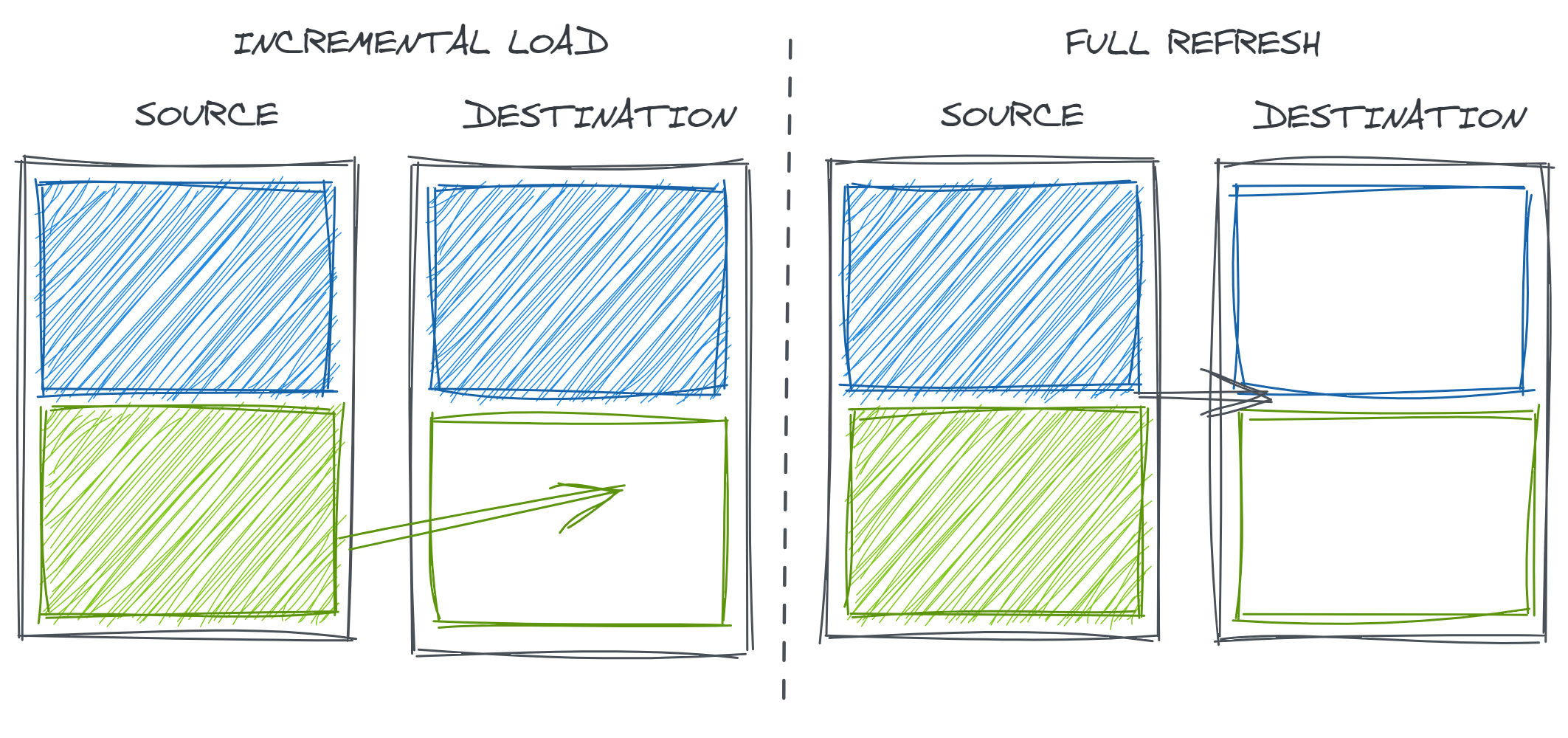
We can see that an incremental load may start with a full load. This load brings over any historical data and the action is shown by the blue box. However, going forward we just bring over a new incremental file. This action is depicted by the green box. Sometimes you might be collecting data from scratch. Thus, there is no history. This is what we are doing with the sample incremental weather data.

A full load means that all data is copied over every scheduled execution of the notebook. The main question to ask the business is “do you need auditing of the data”? If so, we need to keep the full files for each processing day. One great use case for this pattern is critical business process data. Let’s make believe we are a chocolate maker, and we have a set of recipes for creating our chocolate items. We might want to know when the recipe was changed for the almond clusters.

A full load is great for small to medium datasets that do not often change. For extremely large datasets, start with a multi file full load for historical data given the retention period you are looking for. Then going forward, use an incremental file to keep the dataset up to date. In our proof of concept today, we never go back and update history. We will talk about merging datasets with incremental loading in a future thread that will allow for this use case.

Erase Tables

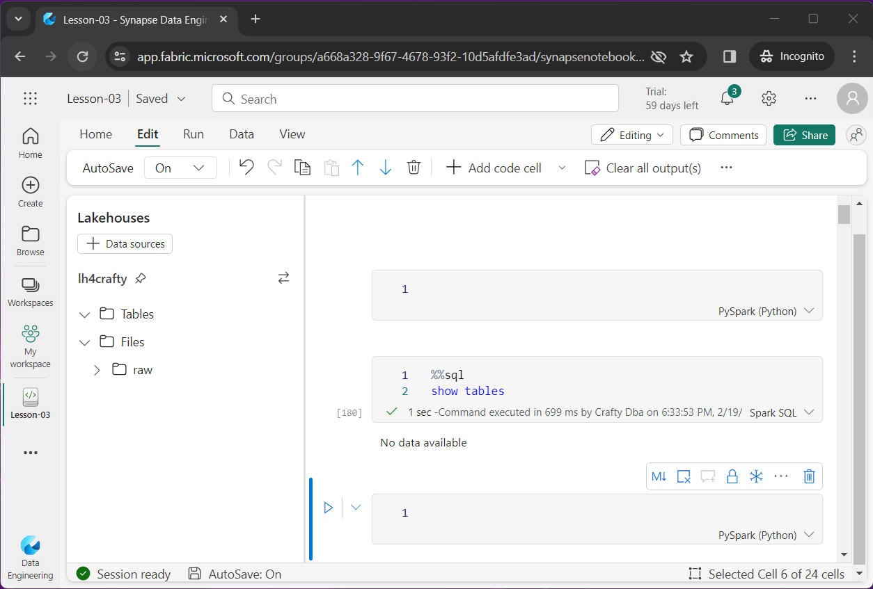
Fabric supplies the data engineer with a parameter cell. We can see that the process variable is currently set to full. However, the Python code in the notebook was built to support the erase, incr and full operations (values). Additionally, we might want to debug variable to be used to optionally display sample data and row counts. This variable supports both true and false values.

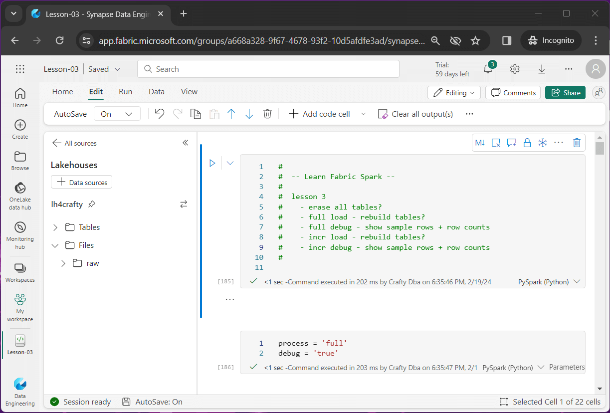
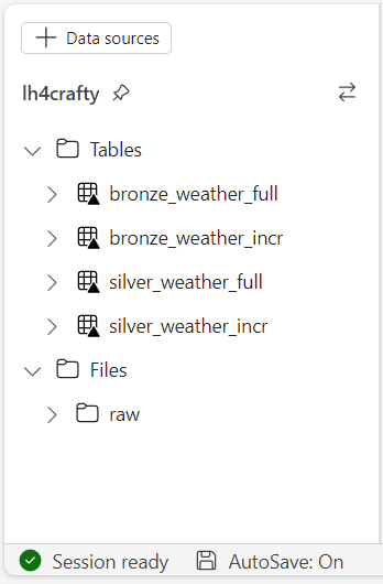
The above image shows the parameter cell we are using in this notebook. The image below shows the end state of the hive catalog. It will have four published tables.

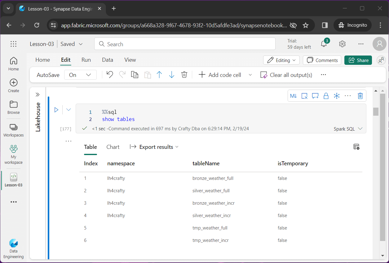
The show tables Spark SQL command lists both permanent and temporary tables.

%%sql
--
-- E2 - show hive + temp tables
--
show tables;

After executing the above Spark SQL statement, we see there are 3 tables in the spark session for each load type: bronze table, silver table and temporary table.

We are going to use the if statement to optionally execute code. If our process variable is set to erase, the following code will execute.

#
# E1 - remove all hive tables
#

if process == 'erase':
  tables = spark.sql('show tables;').collect()
  for table in tables:
    stmt = "drop table " + table.tableName
    ret = spark.sql(stmt)

Here is a quick overview of the above code. First, we grab a DataFrame containing all the Lakehouse tables by calling the spark.sql method with the correct Spark SQL statement. The collect method of the DataFrame returns a list. Then for each table in the list, we execute a drop table command to remove the tables from the hive catalog. The spark variable is just a point to the Spark Session. We will be using this method many times in the future.

The above image shows all the tables that have been removed from the hive catalog.

Full Load

In this section, we are going over code that will be used to create bronze and silver tables using a full load pattern. If we try to create a table when it already exists, the program will error out. The first step in our full load process is to remove the existing bronze and silver tables.

#
# F1 - remove existing tables
#

if process == 'full':
  ret = spark.sql('drop table if exists bronze_weather_full;')
  ret = spark.sql('drop table if exists silver_weather_full;')

The second step in our full load process is to read in the data files as a Spark DataFrame. To fix the data type issue we had in the prior article, we are going to pass a schema definition to the read method. The createOrReplaceTempView method is very powerful. It registers the Spark DataFrame as a temporary view.

#
#  F2 - load data frame
#

# load sub folders into df
if process == 'full':

  # root path
  path = "Files/raw/weather/full/"

  # file schema
  layout = "date timestamp, temp float"

  # load all files
  df = spark.read.format("csv")
    .schema(layout)
    .option("header","true")
    .option("recursiveFileLookup", "true")
    .load(path)

  # convert to view
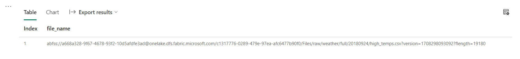
  df.createOrReplaceTempView('tmp_weather_full')

The third step is to use Spark SQL to transform the data. The create table as command allows us to create a hive table with the resulting data from the select statement. Another useful Spark SQL function is input_file_name. The image below shows the full path of the processed file with some additional URL info. The split_part function is very useful when parsing a delimited string and selecting a particular item in an array.

#
#  F3 - create bronze table (all files)
#

# spark sql
stmt = """
  create table bronze_weather_full as
  select
    date as _reading_date,
    temp as _reading_temp,
    current_timestamp() as _load_date,
    split_part(input_file_name(), '/', 9) as _folder_name,
    split_part(split_part(input_file_name(), '/', 10), '?', 1) as _file_name
  from
    tmp_weather_full
"""

# create table?
if process == 'full':
  ret = spark.sql(stmt)

Other than adding additional fields such as folder name, file name, and insert date, the data in the bronze delta table reflects the raw data stored as files and folders. That is about to change when we create the silver delta table.

#
#  F4 - create silver table (lastest files)
#

# spark sql
stmt = """
create table silver_weather_full as
with cte_high_temps as
(
  select *
  from bronze_weather_full as h
  where h._file_name = 'high_temps.csv' and
  h._folder_name = (select max(_folder_name) from bronze_weather_full)
)
, cte_low_temps as
(
  select *
  from bronze_weather_full as l
  where l._file_name = 'low_temps.csv' and
  l._folder_name = (select max(_folder_name) from bronze_weather_full)
)
select
  h._reading_date,
  h._reading_temp as _high_temp,
  l._reading_temp as _low_temp,
  h._load_date,
  h._folder_name,
  h._file_name as _high_file,
  l._file_name as _low_file
from
  cte_high_temps as h
join
  cte_low_temps as l
on
  h._reading_date = l._reading_date
order by
  h._reading_date desc
"""

# create table?
if process == 'full':
  ret = spark.sql(stmt)

We are going to use a common table expression to create two derived tables: cte_high_temps and cte_low_temps. I purposely created the folders using a year, month, and day format. This is a sortable directory. To find the most recent data, we just need to select the data that has the maximum folder value.

Additionally, we want to combine the high temperate and low temperature reading for a given day. I am keeping the source folder name, the high temp file name and the low temp file name as lineage.

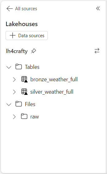
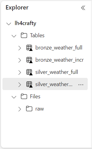
The image below shows the new tables in the hive catalog when executing the Spark Notebook with process equal to full.

Full Table Testing

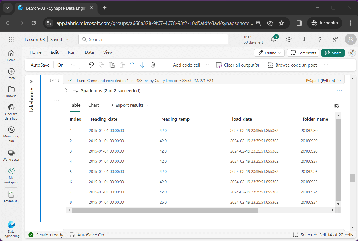
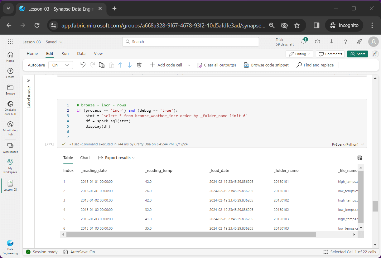
I am going to skip over the code snippets since the complete notebook is enclosed at the end of the article. The first image shows that for a given day, we have 7 entries for high temperatures and 7 entries for low temperatures in the bronze table.

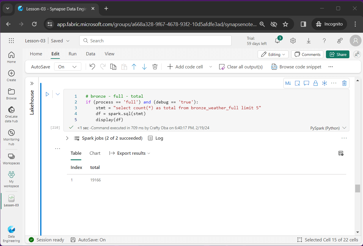
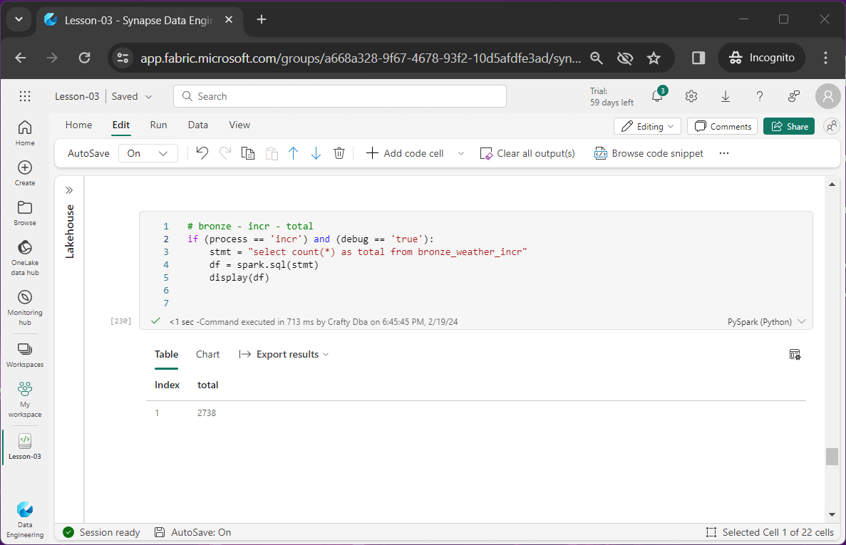
The second image shows the record count from the bronze table. We have a lot of duplicate data.

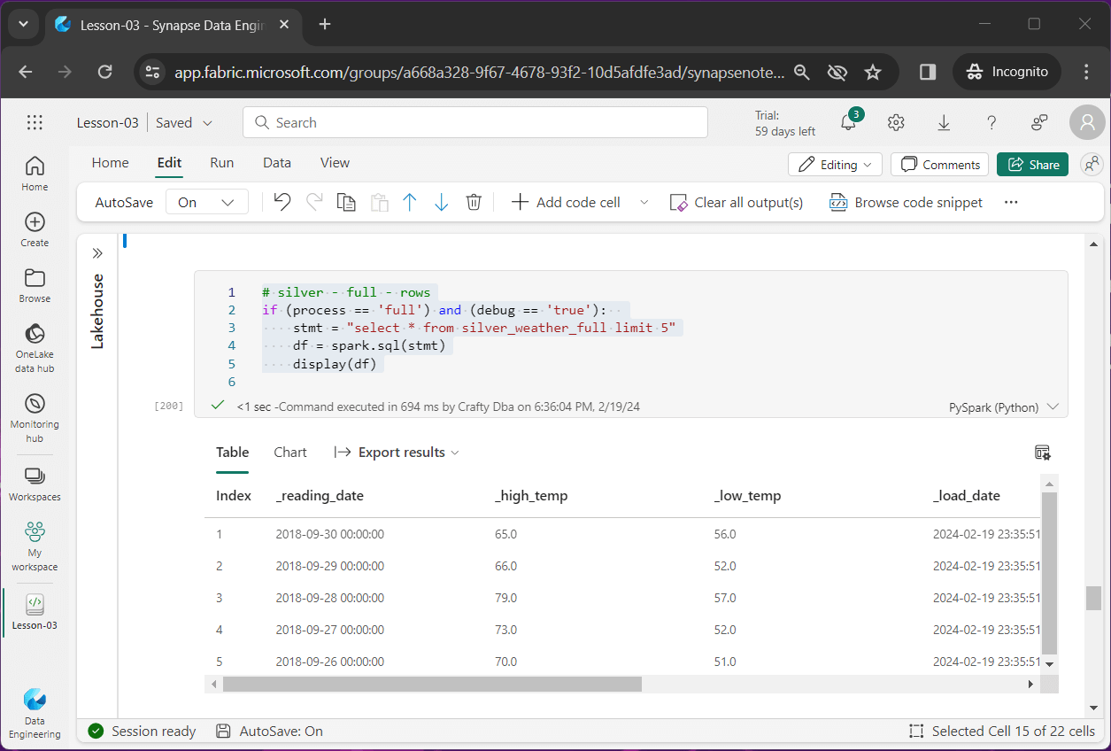
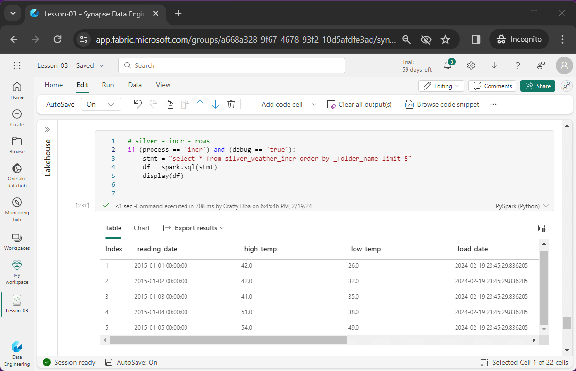
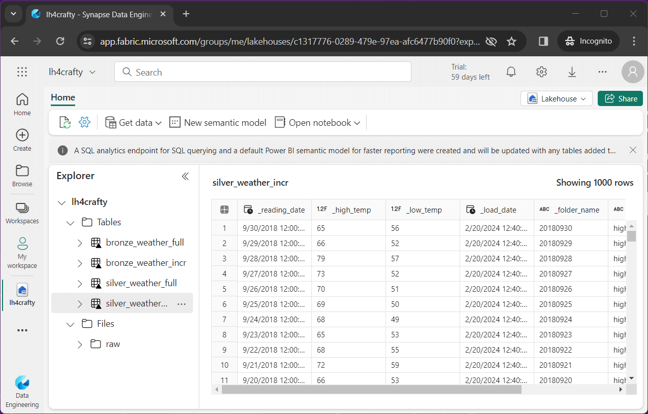
The third image that the silver table has one row per day. That row contains both high and low temperature readings.

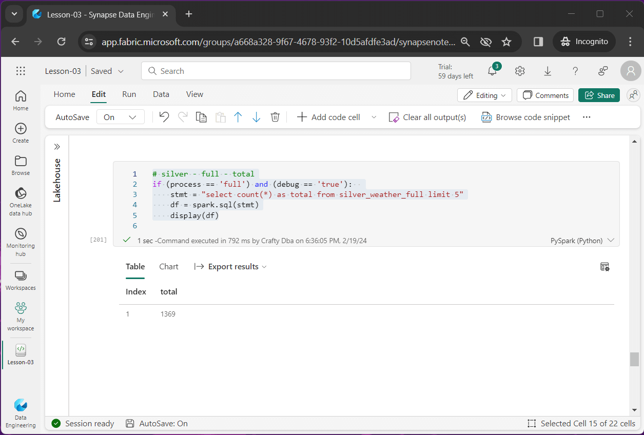
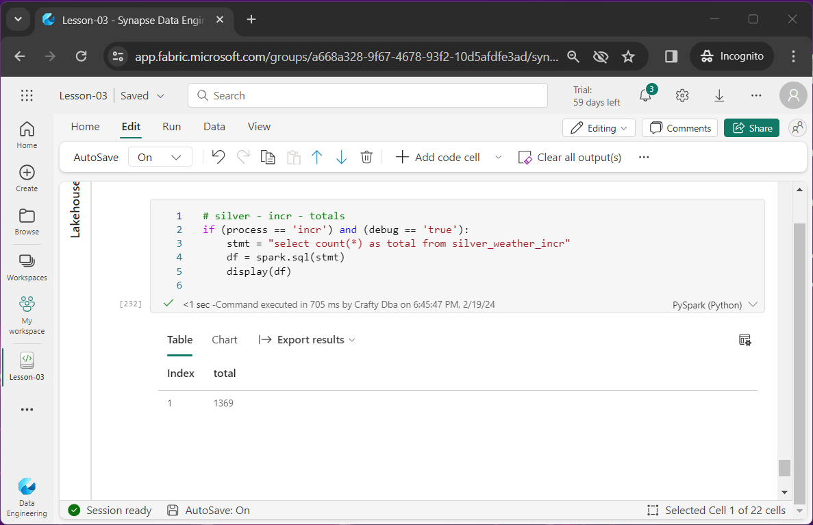
The fourth image shows the silver table has the same number of rows equal to the number of distinct days.

In summary, the bronze table for the full load pattern can be quite large if we decide to keep a lot of historical files.

Incremental Load

In this section, we are going over code that will be used to create bronze and silver tables using an incremental load pattern. There is no historical component since we have data for each day. If we try to create a table when it already exists, the program will error out. The first step in our incremental load process is to remove the existing bronze and silver tables.

#
#  I1 - remove existing tables
#

if process == 'incr':
  ret = spark.sql('drop table if exists bronze_weather_incr;')
  ret = spark.sql('drop table if exists silver_weather_incr;')

The second step in our incremental load process is to read in the data files as a Spark DataFrame. A schema is used to correctly type the data as well as a temporary view. This view allows us to use Spark SQL in steps three and four to transform and create the medallion tables.

#
#  I2 - load data frame
#

# load sub folders into df
if process == 'incr':

  # root path
  path = "Files/raw/weather/incremental/"

  # file schema
  layout = "date timestamp, temp float"

  # load all files
  df = spark.read.format("csv")
    .schema(layout)
    .option("header","true")
    .option("recursiveFileLookup", "true")
    .load(path)

# convert to view
df.createOrReplaceTempView('tmp_weather_incr')

The third step creates the bronze table. Since no filtering and/or transformations are being performed, the code almost matches the full load bronze table code.

#
#  I3 - create bronze table (all files)
#

# spark sql
stmt = """
  create table bronze_weather_incr as
  select
    date as _reading_date,
    temp as _reading_temp,
    current_timestamp() as _load_date,
    split_part(input_file_name(), '/', 9) as _folder_name,
    split_part(split_part(input_file_name(), '/', 10), '?', 1) as _file_name
  from
    tmp_weather_incr
"""

# create table?
if process == 'incr':
  ret = spark.sql(stmt)

The fourth step creates our silver table. Again, we are using a common table expression to separate and combine the high and low temperature data.

#
#  F4 - create silver table (all files)
#

# spark sql
stmt = """
create table silver_weather_incr as
with cte_high_temps as
(
  select *
  from bronze_weather_incr as h
  where h._file_name = 'high_temps.csv'
)
, cte_low_temps as
(
  select *
  from bronze_weather_incr as l
  where l._file_name = 'low_temps.csv'
)
select
  h._reading_date,
  h._reading_temp as _high_temp,
  l._reading_temp as _low_temp,
  h._load_date,
  h._folder_name,
  h._file_name as _high_file,
  l._file_name as _low_file
from
  cte_high_temps as h
join
  cte_low_temps as l
on
  h._reading_date = l._reading_date
order by
  h._reading_date desc
"""

# create table?
if process == 'incr':
  ret = spark.sql(stmt)

The image below shows two new tables for the incremental data.

Incremental Table Testing

I am going to skip over the code snippets since the complete notebook is enclosed at the end of the article. The first image shows that for a given day, we have a sub-folder and two files. One file is for a high temperature reading and one file is for a low temperature reading.

The second image shows that the number of files equals the number of days times two.

The third image shows that the two temperatures have been paired together as one data point.

The fourth image shows that the number of rows is equal to the number of days or 1369.

If we preview the data in the silver incremental table, we can grid looks like the power query interface. The correct data types are assigned to each column (field).

As a consultant, I find a-lot of companies skip steps in regard to system design, commenting code, peer review of code and code testing. Skipping these steps might result in a poor end product.

Going back to the medallion architecture, we can modify the diagram to leave just the files as the data source. This is the only step I did not take in this article. In the next article, we are going to work on scheduling the Spark Notebook with a data pipeline. The SQL analytics endpoint will allow us to expose the existing bronze and silver tables as well as create gold views. This same end point will allow other tools like SSMS to connect to the one lake and use the data.

Summary

Fabric supplies the data engineer with access to the Apache Spark engine to read, transform and write files. Once a file(s) is read into a DataFrame, we can publish a temporary view and perform all the transformation logic using Spark SQL. Yes, you do need to know a language like Python or Scala but remember to test your SQL statements with the %%sql magic command.

Is this code ready for production?

The answer is it all depends. If you are looking for a full load and/or an incremental append pattern, you are all set. This code will work with small to medium datasets. We are rebuilding the delta tables each time from scratch. The amount of processing time will increase linearly with the number of files. There is always the consideration of optimization of large datasets via partitioning or v-order.

In a future article, I will talk about how to handle large datasets with partition and v-order. Additionally, for large datasets we do not want to rebuild the delta table each time. The MERGE command can be used to update the data on a given key.

Let’s think about the sample dataset we were given. It splits data into both high and low temperatures which is crazy. But in real life, a file with longitude, latitude, date, time, and temperature is more appropriate. The sample rate does not matter as long as it is consistent between files. With this new file layout, we can collect data from a multiple set of GPS locations. A simple min and max query by date gives us our final data.

Enclosed is the zip file with the data files and Spark notebook.